Hi,
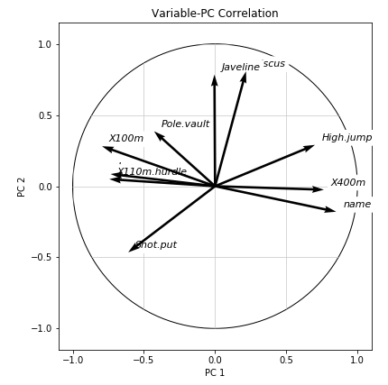
Is it possible to apply mask/clip to grid? Below the the code from matplotlib.
ax_c.grid(clip_path=circ, clip_on=True)
 Read-only archive⌕
Hi,
Is it possible to apply mask/clip to grid? Below the the code from matplotlib.
ax_c.grid(clip_path=circ, clip_on=True)
Hi @grzegorz.malinowski I’m really not entirely sure what it is you want to be able to do. Cna you share a screenshot, or more thorough description?
Ah, no, that is not currently possible. You can set rectangular grid bounds, but not arbitrarily clip like above. No one has ever asked for that before (and I didn’t even know it was possible in MPL).
It’s not critical point, however it could be desirable feature in some cases. Thank you Brian.

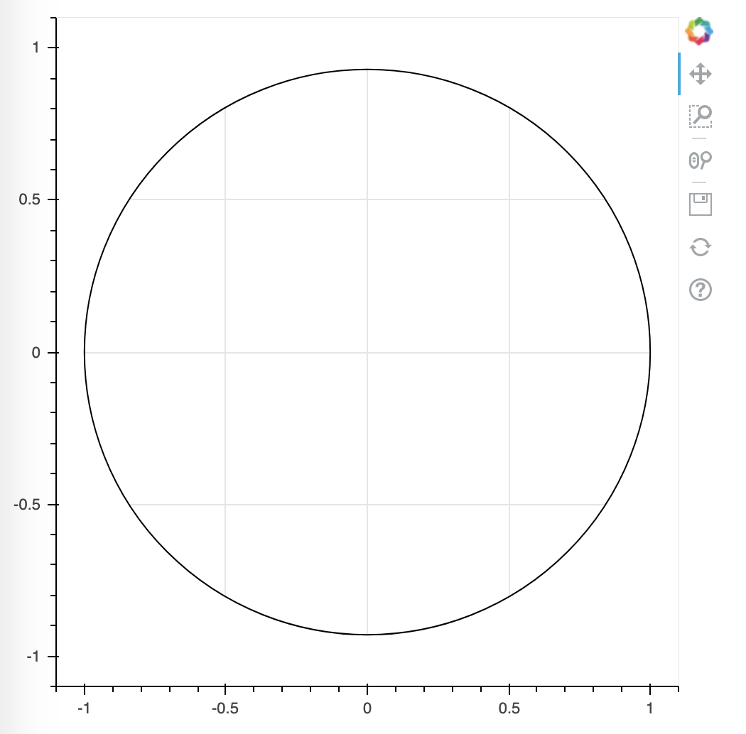
You can achieve something like this with a glyph (or glyphs) that hide parts of the grid you don’t want to see. Here’s a minimal example using an annulus glyph.
#!/usr/bin/env python3
# -*- coding: utf-8 -*-
"""
"""

from bokeh.plotting import figure, show

p = figure(width=500, height=500, x_range=(-1.1,1.1), y_range=(-1.1,1.1))
a = p.annulus(inner_radius=1.0, outer_radius=5.0, fill_color='#ffffff', line_color='#000000')

show(p)
That’s what I’m looking for. Thank you.
I see that you’ve explicitly defined x_range. I was trying range_padding = 5, range_padding_units = 'percent' but it doesn’t work. Is it a bug or I’m doing something wrong?
x_range = DataRange1d(start = -1, end = 1, bounds = (-1, 1), range_padding = 5, range_padding_units = 'percent')
y_range = DataRange1d(start = -1, end = 1, bounds = (-1, 1), range_padding = 5, range_padding_units = 'percent')


p = figure(width=350, height=350, match_aspect=True,
           x_range = x_range, y_range=y_range,
           title="Circle touches all 4 sides of square")
#p.rect(0, 0, 2, 2, line_color='black', alpha=0.0)
#p.circle(x=0, y=0, radius=1, line_color='black',
#          fill_color=None,  radius_units='data')

a = p.annulus(inner_radius=1.0, outer_radius=5.0, fill_color='#ffffff', line_color='#000000')

show(p)I thought about suggesting something like this, but didn’t, because it’s very fragile and requires controlling the ranges explicitly and carefully. You will definitely need to set the range yourself, e.g. to make sure the “masking” glyph stays exactly centered. (I’m assuming that keeping it centered is a requirement)
My interpretation of the bounds property is that it is used for controlling the zooming behavior of the associated data range. By setting the start and end parameters of DataRange1d, you’re controlling the min,max values of the axis range. You should just be able to set these to -1.05 and 1.05, respectively for 5% buffer. I believe my use of the x_range and y_range tuples is equivalent to the DataRange1d with specified values for start and end properties.
One more question. At this stage everything is fine, but when I place LabelSet this glyph-annulus partially masks my labels. How one can manage the order of artists? In MPL there exists zorder param.
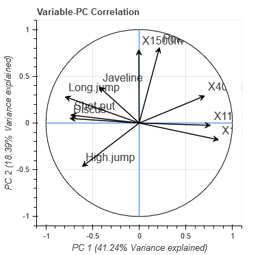
Bokeh renderers have a level property that specifies their RenderLevel. You could potentially “lower” the masking glyph render level, but it’s probably simpler to “raise” the LabelSet render level (to "annotation" or "overlay").
Within a given render level, renderers are drawn in the relative order that they were added (more precisely: in the order they appear in plot.renderers which is in the same order things were added, unless re-arranged manually).
Hi team,
Please let me consult yet another point. Depending on the arrows position one can observe a ‘white background’ under the arrow. Please see CLAY point. The arrow set up is as below. How to fix it?
p_data.add_layout(Arrow(end=VeeHead(size=10, line_color=None), line_width=1.5,
                      x_start=0, y_start=0, x_end='q_x', y_end='q_y', source=source_q))
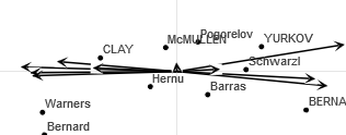
@grzegorz.malinowski seems like a possible bug. Can you see what happens with other arrow head types?
@grzegorz.malinowski I see, can you provide a minimal complete reproducer (e.g with fake or synthetic data) that can be used for investigation?
F = np.array([[-0.0942,  1.1462,  0.5645,  0.0906, -1.3642, -0.7134,  0.3781, -0.083 ,  1.6736,  0.0937],
       [-0.3891,  1.7851, -1.2189,  1.4028,  0.9633,  2.0056,  0.3871, -1.1782,  0.1526, -0.9081],
       [ 0.6545,  1.1888,  0.1762, -2.122 , -0.0983, -0.6161,  0.7389, -1.3435, -0.4317, -0.2837],
       [ 0.4281, -0.3192,  2.2225,  0.7702, -0.4762,  0.1582,  0.5906, -0.2195,  0.278 , -0.3427],
       [ 0.0521, -1.4922, -1.1723, -0.1097,  0.2352,  1.3771, -0.1604, 0.3862,  1.3278, -0.9976],
       [-0.0584, -0.7313, -0.7578,  1.4495, -1.8934,  0.2869, -0.8695, -0.5594,  0.2681, -1.1258],
       [ 1.178 , -0.9476,  0.8069,  0.4122,  2.6783, -0.7022,  0.5449, 0.5567,  0.5671, -1.765 ],
       [ 0.9312,  0.8691,  0.1405,  0.9846,  0.1513,  0.6708,  1.0291, 2.9193, -0.0157,  1.5854],
       [ 0.8738, -0.3042, -0.5913,  0.2527,  0.2792,  0.1388, -0.3926, -1.3029,  1.6988,  1.52  ],
       [ 1.3674, -1.1599, -0.5455, -1.7183, -1.7003,  0.7645,  0.9672, 0.8272,  0.2939, -0.2755],
       [ 2.1734,  0.9319,  0.009 ,  0.7366, -0.5004, -0.1261,  1.0877, -1.0758, -1.3346,  0.1677],
       [-1.6995,  0.8975,  1.5076, -0.8934,  0.0299, -0.1273, -0.0185, 0.0584,  2.1504,  0.6291],
       [-1.633 ,  1.1972,  0.5555, -0.35  , -0.6795,  1.1951, -0.4681, 1.1083, -1.0401, -1.7639],
       [-2.0043, -0.5888, -0.9118,  0.3462,  0.9521, -0.5068,  2.479 , -0.6591, -0.49  ,  0.622 ],
       [-0.9102, -1.5221,  0.8797,  0.6459,  0.0003, -0.3034,  0.4895, 0.6933, -0.9347,  0.6084],
       [-0.6831,  0.2079, -1.7964, -1.1263,  0.0484, -0.8561,  0.4861, 0.209 , -0.4576,  0.6932],
       [-0.2322, -0.6835,  1.5525, -0.2042, -0.4863, -0.175 , -0.0726, -1.027 , -1.4873, -0.4086],
       [-0.1361, -0.8597, -0.1532, -0.9375,  0.8232, -0.5101, -0.8055, -0.472 , -0.1698, -0.5975],
       [-0.6733, -1.0901, -0.7469,  0.8233, -1.0265, -0.5045, -0.661 , -0.0118, -0.7094,  0.9182],
       [ 0.3497,  0.4856, -0.9349, -1.0242,  0.3447, -1.0594, -1.0284, 1.3114,  0.0212, -0.8651],
       [ 0.1055,  0.635 , -0.2674,  1.4975,  0.018 , -2.4509, -1.4247, 0.0718,  0.3313, -0.1059],
       [ 0.2439,  0.9588, -0.0925, -0.2754,  0.7703,  0.2487, -1.5589, 0.4884, -1.4321,  0.8499],
       [ 0.1555, -0.6043,  0.7741, -0.6511,  0.9309,  1.8056, -1.7182, -0.6978, -0.2595,  1.752 ]])

Q = np.array([[ 0.8506, -0.1794,  0.3016,  0.0336,  0.1944,  0.0354,  0.0913, 0.1047,  0.3031,  0.0444],
       [-0.7942,  0.2809, -0.1905, -0.1154, -0.2332, -0.0337,  0.1543, 0.3974,  0.0516,  0.0297],
       [-0.7339,  0.0854,  0.5176,  0.1285,  0.2488, -0.2398,  0.0099, -0.0244, -0.0478,  0.2175],
       [-0.6101, -0.4652,  0.3301,  0.1446, -0.4027, -0.2846, -0.0282, -0.0844,  0.1121, -0.1336],
       [ 0.7016,  0.2902,  0.2835,  0.4308, -0.1039, -0.0493, -0.2861, 0.2336, -0.0822, -0.0342],
       [ 0.7641, -0.0247,  0.4489, -0.0169, -0.2242,  0.0026,  0.3701, 0.0083, -0.1618, -0.0156],
       [-0.7432,  0.0497,  0.1765,  0.395 ,  0.4082,  0.1985,  0.1427, 0.0396, -0.0134, -0.1726],
       [ 0.2173,  0.8075,  0.0941, -0.339 ,  0.2217, -0.3275,  0.0104, -0.0329,  0.0258, -0.1372],
       [-0.4282,  0.3861,  0.6041, -0.3317, -0.1978,  0.3621, -0.1336, -0.0528,  0.0405, -0.0039],
       [-0.0043,  0.7845, -0.2195,  0.448 , -0.2633,  0.0421,  0.1114, -0.1945,  0.1022,  0.0628]])

def plot_bkh(scores=F, loadings=Q, pc_x=1 , pc_y=2):

    tools = 'pan, box_zoom, reset, save'

    data = {'x_data': scores[:,(pc_x-1)],
            'y_data': scores[:,(pc_y-1)],}
    source = ColumnDataSource(data=data)


    data_q = {'q_x': Q[:,(pc_x-1)],
              'q_y': Q[:,(pc_y-1)],}
    source_q = ColumnDataSource(data=data_q)


    p_data = figure(plot_height=400, plot_width=600,
                    tools=tools, match_aspect=False)


    p_data.circle('x_data', 'y_data', source=source, size=6, line_color='white', fill_color='black')

    p_data.add_layout(Arrow(end=VeeHead(size=10), line_width=1.5,
                          x_start=0, y_start=0, x_end='q_x', y_end='q_y', source=source_q))

    show(p_data)

plot_bkh(pc_x=1 , pc_y=10)@grzegorz.malinowski great can you make that complete (e.g. missing imports) and file a new issue at Issues · bokeh/bokeh · GitHub (please include version info, etc)
Sure, having no experience with that, hope everything is fine. DONE

End of archived discussion · Replies are disabled