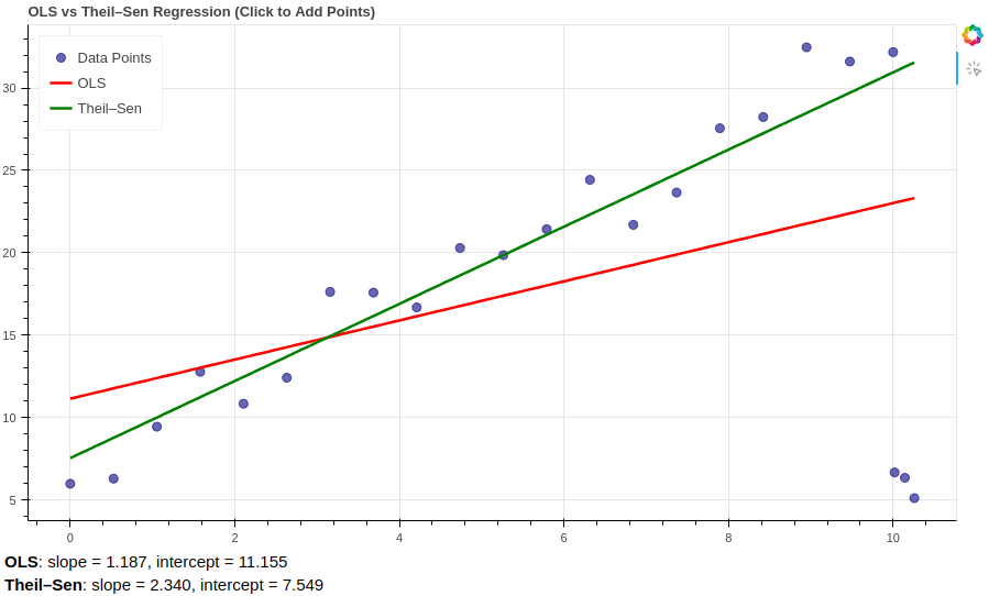
This chart demonstrates the difference between classic OLS linear regression and robust Theil–Sen estimation in the presence of noisy or outlier data. Users can click anywhere on the canvas to add new data points. Both regression lines are recalculated live on the fly, and the current slope and intercept values for each model are displayed below the plot. Bokeh is also nice for educational demos and statistical intuition building.
CustomJS:
from bokeh.plotting import figure, output_file, save
from bokeh.models import ColumnDataSource, CustomJS, Div
from bokeh.layouts import column
import numpy as np
from scipy.stats import linregress

# 🎲 Natural-looking linear data
np.random.seed(42)
x = np.linspace(0, 10, 20)
noise = np.random.normal(0, 2, len(x))
y = 3 * x + 5 + noise

# === Initial OLS ===
slope, intercept, *_ = linregress(x, y)
x_range = np.linspace(min(x), max(x), 100)
y_ols = slope * x_range + intercept

# === ColumnDataSources ===
source = ColumnDataSource(data=dict(x=x.tolist(), y=y.tolist()))
ols_source = ColumnDataSource(data=dict(x=x_range.tolist(), y=y_ols.tolist()))
ts_source = ColumnDataSource(data=dict(x=x_range.tolist(), y=y_ols.tolist()))  # dummy, updated in JS

# === Div for displaying slope/intercept
info_div = Div(text="Click on plot to add point & update trendlines.", styles={"font-size": "15px", "color": "black"})

# === Plot setup (light theme)
p = figure(
    title="OLS vs Theil–Sen Regression (Click to Add Points)",
    tools="tap",
    width=900,
    height=500
)

p.circle('x', 'y', source=source, size=8, color="navy", alpha=0.6, legend_label="Data Points")
p.line('x', 'y', source=ols_source, line_width=2.5, color="red", legend_label="OLS")
p.line('x', 'y', source=ts_source, line_width=2.5, color="green", legend_label="Theil–Sen")
p.legend.location = "top_left"

# === JS Callback
callback = CustomJS(args=dict(source=source, ols=ols_source, ts=ts_source, info=info_div), code=""" const data = source.data; const x = data.x; const y = data.y; // Add new point x.push(cb_obj.x); y.push(cb_obj.y); const n = x.length; // --- OLS --- let sum_x = 0, sum_y = 0, sum_xy = 0, sum_xx = 0; for (let i = 0; i < n; i++) { sum_x += x[i]; sum_y += y[i]; sum_xy += x[i] * y[i]; sum_xx += x[i] * x[i]; } const slope_ols = (n * sum_xy - sum_x * sum_y) / (n * sum_xx - sum_x * sum_x); const intercept_ols = (sum_y - slope_ols * sum_x) / n; // --- Theil–Sen --- let slopes = []; for (let i = 0; i < n; i++) { for (let j = i + 1; j < n; j++) { const dx = x[j] - x[i]; const dy = y[j] - y[i]; if (dx !== 0) slopes.push(dy / dx); } } slopes.sort((a, b) => a - b); const medianSlope = slopes.length % 2 === 1 ? slopes[Math.floor(slopes.length / 2)] : (slopes[slopes.length / 2 - 1] + slopes[slopes.length / 2]) / 2; let intercepts = []; for (let i = 0; i < n; i++) { intercepts.push(y[i] - medianSlope * x[i]); } intercepts.sort((a, b) => a - b); const medianIntercept = intercepts.length % 2 === 1 ? intercepts[Math.floor(intercepts.length / 2)] : (intercepts[intercepts.length / 2 - 1] + intercepts[intercepts.length / 2]) / 2; // --- Generate Trendlines --- const x_min = Math.min(...x); const x_max = Math.max(...x); const steps = 100; const step = (x_max - x_min) / (steps - 1); const x_vals = [], y_ols_vals = [], y_ts_vals = []; for (let i = 0; i < steps; i++) { const xi = x_min + i * step; x_vals.push(xi); y_ols_vals.push(slope_ols * xi + intercept_ols); y_ts_vals.push(medianSlope * xi + medianIntercept); } ols.data = { x: x_vals, y: y_ols_vals }; ts.data = { x: x_vals, y: y_ts_vals }; // --- Update Info Box --- info.text = ` <b>OLS</b>: slope = ${slope_ols.toFixed(3)}, intercept = ${intercept_ols.toFixed(3)}<br> <b>Theil–Sen</b>: slope = ${medianSlope.toFixed(3)}, intercept = ${medianIntercept.toFixed(3)} `; source.change.emit(); ols.change.emit(); ts.change.emit(); """)
# Hook up callback
p.js_on_event('tap', callback)

# === Save HTML
output_file("scatter_with_slope_text.html")
save(column(p, info_div))
Bokeh Server:
from bokeh.plotting import figure, curdoc
from bokeh.models import ColumnDataSource, Div
from bokeh.layouts import column
import numpy as np
from scipy.stats import linregress, theilslopes

# Initial data
np.random.seed(42)
x = np.linspace(0, 10, 20)
y = 3 * x + 5 + np.random.normal(0, 2, len(x))

source = ColumnDataSource(data=dict(x=list(x), y=list(y)))
ols_source = ColumnDataSource(data=dict(x=[], y=[]))
ts_source = ColumnDataSource(data=dict(x=[], y=[]))
info_div = Div(text="", styles={"font-size": "15px"})

def update_regression():
    x = np.array(source.data['x'])
    y = np.array(source.data['y'])

    # OLS
    slope_ols, intercept_ols, *_ = linregress(x, y)
    x_fit = np.linspace(min(x), max(x), 100)
    y_fit_ols = slope_ols * x_fit + intercept_ols
    ols_source.data = dict(x=x_fit, y=y_fit_ols)

    # Theil–Sen
    slope_ts, intercept_ts, *_ = theilslopes(y, x)
    y_fit_ts = slope_ts * x_fit + intercept_ts
    ts_source.data = dict(x=x_fit, y=y_fit_ts)

    info_div.text = (
        f"<b>OLS</b>: slope = {slope_ols:.3f}, intercept = {intercept_ols:.3f}<br>"
        f"<b>Theil–Sen</b>: slope = {slope_ts:.3f}, intercept = {intercept_ts:.3f}"
    )

update_regression()

# Plot setup
p = figure(title="OLS vs Theil–Sen (Click to Add)", tools="tap", width=900, height=500)
p.circle('x', 'y', source=source, size=8, color="navy", alpha=0.6, legend_label="Points")
p.line('x', 'y', source=ols_source, line_width=2.5, color="red", legend_label="OLS")
p.line('x', 'y', source=ts_source, line_width=2.5, color="green", legend_label="Theil–Sen")
p.legend.location = "top_left"

# Callback on click
def on_tap(event):
    new_data = dict(x=source.data['x'] + [event.x], y=source.data['y'] + [event.y])
    source.data = new_data
    update_regression()

p.on_event('tap', on_tap)

curdoc().add_root(column(p, info_div))
curdoc().title = "Regression Comparison"