A custom BokehJS extension that brings interactive 3D globe visualization to Bokeh. Plot gridded data (temperature, precipitation, etc.) on a rotating sphere with coastlines, country borders, and multi-layer overlays including scatter points, 3D bars, flight routes, and satellite trajectories. Features drag-to-rotate, auto-rotation, optional Phong lighting for realistic shading, integrated colorbar, and smart tooltips that work across all data layers.
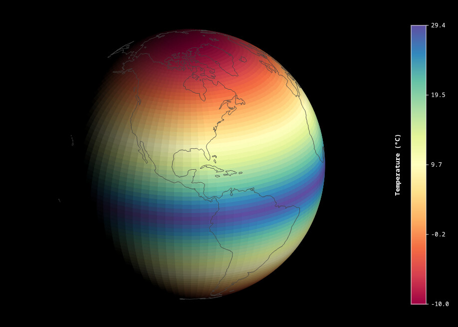
![]() Spherical projection with depth sorting
Spherical projection with depth sorting
![]()
![]() Drag rotation/tilt, scroll zoom, auto-rotation
Drag rotation/tilt, scroll zoom, auto-rotation
![]() Auto-loaded Natural Earth coastlines & borders
Auto-loaded Natural Earth coastlines & borders
![]()
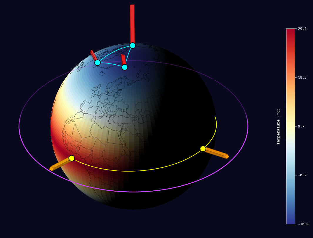
![]() Scatter points, 3D bars, lines, 3D trajectories
Scatter points, 3D bars, lines, 3D trajectories
![]()
![]() Optional lighting (azimuth/elevation/intensity)
Optional lighting (azimuth/elevation/intensity)
![]() 30+ color palettes with integrated colorbar
30+ color palettes with integrated colorbar
![]() Multi-layer tooltips (grid values, labels, heights)
Multi-layer tooltips (grid values, labels, heights)
Free and open source code is here:
Simply download the folder, install bokeh numpy pandas and xarray, and run the several examples, includingd in bokeh_gridded_sphere_examples.py.
Simple example:
from gridded_sphere_py import GriddedSphere
from bokeh.plotting import show
import numpy as np
# Create grid
n_lat = 60; n_lon = 120;lons = np.linspace(-180, 180, n_lon);lats = np.linspace(-90, 90, n_lat)
lons_grid, lats_grid = np.meshgrid(lons, lats)
# Temperature pattern
values = 30 - 50 * np.abs(lats_grid) / 90;values += 10 * np.sin(np.radians(lons_grid) * 3) * np.cos(np.radians(lats_grid) * 2)
# Create sphere
sphere1 = GriddedSphere(
    lons=lons_grid.flatten().tolist(),
    lats=lats_grid.flatten().tolist(),
    values=values.flatten().tolist(),
    n_lat=n_lat,
    n_lon=n_lon,
    palette='Spectral',
    autorotate = True
)
show(sphere1)
from points import cities
from bokeh.plotting import show
from gridded_sphere_py import GriddedSphere
import numpy as np

# Create realistic Earth-like gridded data
n_lat = 40
n_lon = 80

lats = np.linspace(-90, 90, n_lat)
lons = np.linspace(-180, 180, n_lon)
lon_grid, lat_grid = np.meshgrid(lons, lats)

# Temperature-like pattern
temperature = 25 - 35 * np.abs(np.sin(np.radians(lat_grid))) + 5 * np.cos(np.radians(lon_grid) * 2)

earthquakes = [
    # Pacific Ring of Fire
    {'lon': 142.3, 'lat': 38.3, 'size': 16, 'color': '#ff0000',
     'border_color': '#000000', 'border_width': 2, 'label': 'Japan M7.3 (2022)'},
    {'lon': 143.9, 'lat': 37.0, 'size': 18, 'color': '#ff0000',
     'border_color': '#000000', 'border_width': 2, 'label': 'Fukushima M7.4 (2022)'},
    {'lon': -103.3, 'lat': 19.4, 'size': 15, 'color': '#ff3300',
     'border_color': '#000000', 'border_width': 2, 'label': 'Mexico M7.1 (2022)'},
    {'lon': -72.2, 'lat': -33.0, 'size': 14, 'color': '#ff6600',
     'border_color': '#000000', 'border_width': 2, 'label': 'Chile M6.9 (2023)'},
    {'lon': 174.0, 'lat': -41.7, 'size': 15, 'color': '#ff9900',
     'border_color': '#000000', 'border_width': 2, 'label': 'New Zealand M7.2 (2021)'},
    {'lon': -155.5, 'lat': 19.4, 'size': 13, 'color': '#ffcc00',
     'border_color': '#000000', 'border_width': 2, 'label': 'Hawaii M6.8 (2022)'},

    # Turkey-Syria
    {'lon': 37.2, 'lat': 37.2, 'size': 20, 'color': '#ff0000',
     'border_color': '#000000', 'border_width': 3, 'label': 'Turkey M7.8 (2023)'},
    {'lon': 37.0, 'lat': 38.0, 'size': 18, 'color': '#ff0000',
     'border_color': '#000000', 'border_width': 3, 'label': 'Turkey M7.5 (2023)'},

    # Indonesia & Philippines
    {'lon': 119.8, 'lat': -1.3, 'size': 14, 'color': '#ff6600',
     'border_color': '#000000', 'border_width': 2, 'label': 'Indonesia M7.0 (2023)'},
    {'lon': 126.4, 'lat': 10.7, 'size': 13, 'color': '#ff9900',
     'border_color': '#000000', 'border_width': 2, 'label': 'Philippines M6.9 (2023)'},

    # South Pacific
    {'lon': -178.3, 'lat': -18.2, 'size': 17, 'color': '#ff3300',
     'border_color': '#000000', 'border_width': 2, 'label': 'Fiji M7.6 (2024)'},
    {'lon': 166.9, 'lat': -14.9, 'size': 16, 'color': '#ff6600',
     'border_color': '#000000', 'border_width': 2, 'label': 'Vanuatu M7.3 (2023)'},

    # Alaska
    {'lon': -149.0, 'lat': 61.3, 'size': 14, 'color': '#ff9900',
     'border_color': '#000000', 'border_width': 2, 'label': 'Alaska M7.0 (2023)'},

    # Afghanistan
    {'lon': 70.0, 'lat': 35.0, 'size': 13, 'color': '#ffcc00',
     'border_color': '#000000', 'border_width': 2, 'label': 'Afghanistan M6.8 (2023)'},

    # Morocco
    {'lon': -8.5, 'lat': 31.1, 'size': 15, 'color': '#ff6600',
     'border_color': '#000000', 'border_width': 2, 'label': 'Morocco M6.8 (2023)'},
]

sphere_scatter = GriddedSphere(
    lons=lon_grid.flatten().tolist(),
    lats=lat_grid.flatten().tolist(),
    values=temperature.flatten().tolist(),
    n_lat=n_lat,
    n_lon=n_lon,
    palette='terrain',
    width=900,
    height=900,
    rotation=145,
    tilt=20,
    zoom=0.8,
    autorotate=False,
    scatter_data=earthquakes,
    show_colorbar=True,
    background_color='#000000',
    show_coastlines=True,
    coastline_color='#666666',
    coastline_width=0.6,
    show_countries=True,
    country_color='#444444',
    country_width=0.3
)

show(sphere_scatter)
np.random.seed(42)
n_bars = 30
random_bars = []

for i in range(n_bars):
    lon = np.random.uniform(-180, 180)
    lat = np.random.uniform(-60, 60)
    height = np.random.uniform(50, 800)

    # Color based on hemisphere
    if lat > 0:
        color = '#ff6b6b'  # Northern hemisphere - red
    else:
        color = '#4ecdc4'  # Southern hemisphere - cyan

    random_bars.append({
        'lon': lon,
        'lat': lat,
        'height': height,
        'color': color,
        'label': f'Lat: {lat:.1f}, Height: {height:.0f}'
    })

sphere2 = GriddedSphere(
    lons=lon_grid.flatten().tolist(),
    lats=lat_grid.flatten().tolist(),
    values=temperature.flatten().tolist(),
    n_lat=n_lat,
    n_lon=n_lon,
    palette='inferno',
    bar_data=random_bars,
)
show(sphere2)
from bokeh.plotting import show
from bokeh.layouts import column
from gridded_sphere_py import GriddedSphere
import numpy as np

# Create some sample gridded data
n_lat = 100
n_lon = 100

lats = np.linspace(-90, 90, n_lat)
lons = np.linspace(-180, 180, n_lon)
lon_grid, lat_grid = np.meshgrid(lons, lats)

# Create realistic Earth-like data
# Temperature gradient: hot at equator, cold at poles
temperature = 30 - 40 * np.abs(np.sin(np.radians(lat_grid)))

# === Example 1: Classic day-night terminator ===
# Light from the right side (like afternoon sun)
sphere1 = GriddedSphere(
    lons=lon_grid.flatten().tolist(),
    lats=lat_grid.flatten().tolist(),
    values=temperature.flatten().tolist(),
    n_lat=n_lat,
    n_lon=n_lon,
    palette='Spectral',
    width=800,
    height=800,
    rotation=0,
    tilt=-23.5,  # Earth's axial tilt
    zoom=0.8,
    autorotate=False,
    enable_lighting=True,
    light_azimuth=135,    # Light from upper right
    light_elevation=25,    # 45 degrees above horizon
    light_intensity=1.2,   # Strong directional light
    ambient_light=0,    # Some ambient illumination
    show_colorbar=True,
    colorbar_title='Temperature (°C)',
    background_color='#000000',
    show_coastlines=True,
    coastline_color='#414141',
    coastline_width=0.9
)

show(sphere1)
import numpy as np
from gridded_sphere_py import GriddedSphere
from bokeh.io import show
def make_ring(inclination_deg, raan_deg, altitude, n=300):
inc = np.radians(inclination_deg)
raan = np.radians(raan_deg)
t = np.linspace(0, 2 * np.pi, n, endpoint=False)
x = np.cos(t)
y = np.sin(t) * np.cos(inc)
z = np.sin(t) * np.sin(inc)
x2 = x * np.cos(raan) - y * np.sin(raan)
y2 = x * np.sin(raan) + y * np.cos(raan)
lon = np.degrees(np.arctan2(y2, x2))
lat = np.degrees(np.arcsin(np.clip(z, -1, 1)))
# Split into two continuous segments at the lon wraparound
# Find where lon jumps (the discontinuity from +180 to -180)
dlon = np.diff(lon)
wrap_idx = np.where(np.abs(dlon) > 180)[0]
coords = [{'lon': float(lon[i]), 'lat': float(lat[i]), 'altitude': altitude} for i in range(n)]
if len(wrap_idx) == 0:
# No wrap, single segment
return [coords]
else:
# Split at each wrap point into separate segments
segments = []
prev = 0
for idx in wrap_idx:
segments.append(coords[prev:idx + 1])
prev = idx + 1
segments.append(coords[prev:])
# Close the ring: connect last segment back to first point
segments[-1].append(coords[0])
return segments
def add_ring(trajectories, inclination_deg, raan_deg, altitude, color):
segments = make_ring(inclination_deg, raan_deg, altitude)
for seg in segments:
trajectories.append({
'coords': seg,
'color': color,
'width': 2.5,
'show_points': False,
})
trajectories = []
add_ring(trajectories, inclination_deg=0, raan_deg=0, altitude=472, color='#cc44ff')
add_ring(trajectories, inclination_deg=51.6, raan_deg=0, altitude=140, color='#00ffff')
add_ring(trajectories, inclination_deg=98, raan_deg=60, altitude=225, color='#ffdd00')
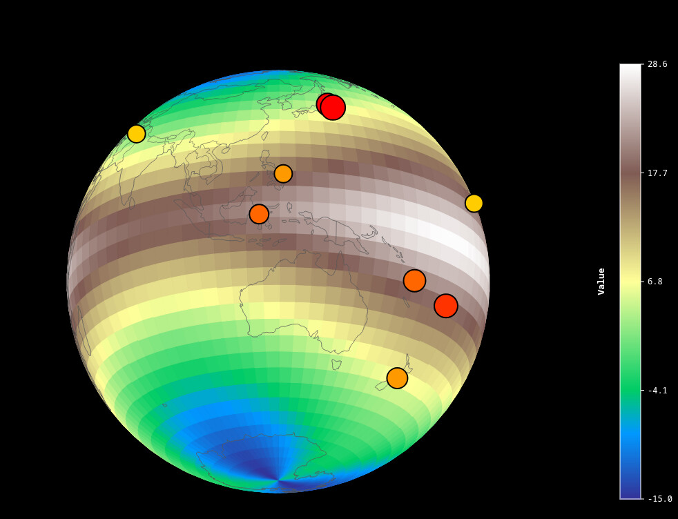
# Research stations (scatter)
research_stations = [
# Arctic
{'lon': -51.7, 'lat': 64.2, 'size': 10, 'color': '#00ffff',
'border_color': '#000000', 'border_width': 2, 'label': 'Greenland Station'},
{'lon': 11.9, 'lat': 78.9, 'size': 10, 'color': '#00ffff',
'border_color': '#000000', 'border_width': 2, 'label': 'Svalbard Station'},
{'lon': -133.5, 'lat': 68.3, 'size': 10, 'color': '#00ffff',
'border_color': '#000000', 'border_width': 2, 'label': 'Alaska Station'},
# Tropical
{'lon': -3.0, 'lat': 0.0, 'size': 10, 'color': '#ffff00',
'border_color': '#000000', 'border_width': 2, 'label': 'Atlantic Equator'},
{'lon': 160.0, 'lat': 0.0, 'size': 10, 'color': '#ffff00',
'border_color': '#000000', 'border_width': 2, 'label': 'Pacific Equator'},
{'lon': 102.0, 'lat': 3.0, 'size': 10, 'color': '#ffff00',
'border_color': '#000000', 'border_width': 2, 'label': 'Borneo Station'},
# Antarctic
{'lon': 0.0, 'lat': -75.0, 'size': 10, 'color': '#ffffff',
'border_color': '#000000', 'border_width': 2, 'label': 'Antarctic Station 1'},
{'lon': 166.7, 'lat': -77.8, 'size': 10, 'color': '#ffffff',
'border_color': '#000000', 'border_width': 2, 'label': 'McMurdo Station'},
]
# Communication networks (lines)
data_links = [
{
'coords': [
[-51.7, 64.2], # Greenland
[11.9, 78.9], # Svalbard
[-133.5, 68.3], # Alaska
[-51.7, 64.2], # Back to Greenland
],
'color': '#00ffff',
'width': 2,
'label': 'Arctic Network'
},
{
'coords': [
[-3.0, 0.0], # Atlantic
[102.0, 3.0], # Borneo
[160.0, 0.0], # Pacific
],
'color': '#ffff00',
'width': 2,
'label': 'Tropical Network'
},
{
'coords': [
[0.0, -75.0], # Antarctic 1
[166.7, -77.8], # McMurdo
],
'color': '#ffffff',
'width': 2,
'label': 'Antarctic Network'
},
]
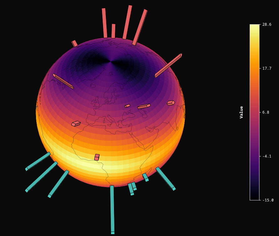
# Temperature anomaly bars
temperature_anomalies = [
{'lon': -51.7, 'lat': 64.2, 'height': 220, 'width': 2, 'color': '#ff4444',
'border_color': '#880000', 'label': 'Greenland: +2.2°C'},
{'lon': 11.9, 'lat': 78.9, 'height': 260, 'width': 2, 'color': '#ff2222',
'border_color': '#880000', 'label': 'Svalbard: +2.6°C'},
{'lon': -133.5, 'lat': 68.3, 'height': 630, 'width': 2, 'color': '#ff3333',
'border_color': '#880000', 'label': 'Alaska: +2.3°C'},
{'lon': -3.0, 'lat': 0.0, 'height': 410, 'width': 2, 'color': '#ffaa00',
'border_color': '#884400', 'label': 'Atlantic: +1.1°C'},
{'lon': 160.0, 'lat': 0.0, 'height': 595, 'width': 2, 'color': '#ffcc00',
'border_color': '#884400', 'label': 'Pacific: +0.95°C'},
{'lon': 102.0, 'lat': 3.0, 'height': 430, 'width': 2, 'color': '#ff9900',
'border_color': '#884400', 'label': 'Borneo: +1.3°C'},
{'lon': 0.0, 'lat': -75.0, 'height': 190, 'width': 2, 'color': '#4444ff',
'border_color': '#000088', 'label': 'Antarctic: +1.9°C'},
{'lon': 166.7, 'lat': -77.8, 'height': 510, 'width': 2, 'color': '#3333ff',
'border_color': '#000088', 'label': 'McMurdo: +2.1°C'},
]
sphere_combined = GriddedSphere(
lons=lon_grid.flatten().tolist(),
lats=lat_grid.flatten().tolist(),
values=temperature.flatten().tolist(),
n_lat=n_lat,
n_lon=n_lon,
palette='RdYlBu_r',
width=950,
height=950,
rotation=-135,
tilt=-35,
zoom=0.7,
autorotate=False,
scatter_data=research_stations,
line_data=data_links,
bar_data=temperature_anomalies,
show_colorbar=True,
colorbar_title='Temperature (°C)',
background_color='#0a0a1e',
show_coastlines=True,
coastline_color='#000000',
coastline_width=0.5,
show_countries=True,
country_color='#000000',
country_width=0.3,
enable_lighting=True,
light_azimuth=135, # Light from upper right
light_elevation=25, # 45 degrees above horizon
light_intensity=1.2, # Strong directional light
ambient_light=0,
trajectory_data=[trajectories[0],trajectories[1]],
)
show(sphere_combined)
Interactive with CustomJS:
########## CUSTOMJS INTERACTIONS ##############
import numpy as np
from bokeh.plotting import figure, show
from bokeh.layouts import column, row
from bokeh.models import (
Slider, Button, Div, CustomJS, ColumnDataSource, Range1d
)
from gridded_sphere_py import GriddedSphere
# ---------------------------------------------------------------------------
# Grid setup
# ---------------------------------------------------------------------------
n_lat = 100
n_lon = 100
lats = np.linspace(-90, 90, n_lat)
lons = np.linspace(-180, 180, n_lon)
lon_grid, lat_grid = np.meshgrid(lons, lats)
# ---------------------------------------------------------------------------
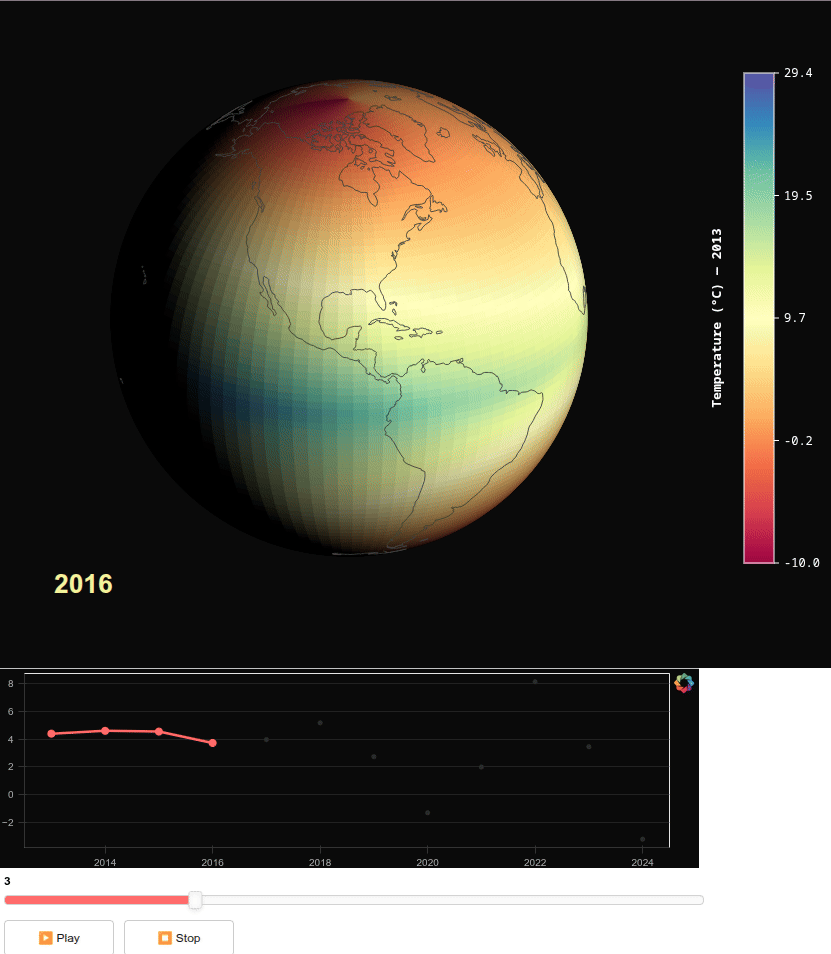
# 12 years of temperature data (2013–2024)
# ---------------------------------------------------------------------------
years = list(range(2013, 2025))
n_years = len(years)
all_values = []
yearly_mean = []
for i in range(n_years):
base = 30 - 40 * np.abs(np.sin(np.radians(lat_grid)))
trend = 0.15 * i
noise = 1.5 * i**2 *np.sin(np.radians(lat_grid * 1.3 + i * 37)) \
* np.cos(np.radians(lon_grid * 0.8 + i * 53))
temp = base + trend + noise
all_values.append(temp.flatten().tolist())
yearly_mean.append(float(np.mean(temp)))
# ---------------------------------------------------------------------------
# Sphere with initial data
# ---------------------------------------------------------------------------
sphere = GriddedSphere(
lons=lon_grid.flatten().tolist(),
lats=lat_grid.flatten().tolist(),
values=all_values[0],
n_lat=n_lat,
n_lon=n_lon,
palette='Spectral',
width=700,
height=700,
rotation=0,
tilt=-23.5,
zoom=0.8,
autorotate=False,
enable_lighting=True,
light_azimuth=135,
light_elevation=25,
light_intensity=1.2,
ambient_light=0.0,
show_colorbar=True,
colorbar_title=f'Temperature (°C) — {years[0]}',
background_color='#0a0a0a',
show_coastlines=True,
coastline_color='#414141',
coastline_width=0.9,
)
# Store all years of data in sphere.tags (THIS IS THE KEY!)
sphere.tags = all_values
# ---------------------------------------------------------------------------
# Timeseries plot
# ---------------------------------------------------------------------------
ts_source = ColumnDataSource(data={
'x': [years[0]],
'y': [yearly_mean[0]],
})
# Ghost dots (all years, faint)
ghost_source = ColumnDataSource(data={
'x': years,
'y': yearly_mean,
})
ts_fig = figure(
width=700, height=200,
x_range=Range1d(2012.5, 2024.5),
y_range=Range1d(min(yearly_mean) - 0.6, max(yearly_mean) + 0.6),
tools='',
background_fill_color='#0a0a0a',
border_fill_color='#0a0a0a',
)
ts_fig.xgrid.visible = False
ts_fig.ygrid.grid_line_color = '#222222'
ts_fig.axis.axis_label_text_color = '#aaaaaa'
ts_fig.axis.major_label_text_color = '#aaaaaa'
ts_fig.axis.axis_line_color = '#333333'
ts_fig.axis.major_tick_line_color = '#333333'
ts_fig.axis.minor_tick_line_color = None
ts_fig.axis.axis_label_text_font_size = '11px'
ts_fig.axis.major_label_text_font_size = '10px'
# Ghost points
ts_fig.circle('x', 'y', source=ghost_source, size=5, color='#2a2a2a', line_color=None)
# Animated line + active dots
ts_fig.line('x', 'y', source=ts_source, color='#ff6b6b', line_width=2.5)
ts_fig.circle('x', 'y', source=ts_source, size=7, color='#ff6b6b', line_color='#ff6b6b')
# ---------------------------------------------------------------------------
# Year label
# ---------------------------------------------------------------------------
year_label = Div(text=f"""
<div style="
position: relative;
top: -400px;
left: 50px;
background: transparent !important;
">
<div style="font-size: 2.2em; font-weight: 900; color: #fcf18d; margin-bottom:0.28em;">{years[0]}</div>
</div>
""")
# ---------------------------------------------------------------------------
# Slider
# ---------------------------------------------------------------------------
slider = Slider(
start=0, end=n_years - 1, value=0, step=1,
width=700, title='',
bar_color='#ff6b6b',
)
# ---------------------------------------------------------------------------
# Play / Stop
# ---------------------------------------------------------------------------
play_btn = Button(label='▶ Play', button_type='default', width=110, height=36)
stop_btn = Button(label='⏹ Stop', button_type='default', width=110, height=36)
# ---------------------------------------------------------------------------
# CustomJS: slider change -> update sphere + timeseries + label
# FORCE UPDATE by changing colorbar_title which triggers re-render
# ---------------------------------------------------------------------------
update_cb = CustomJS(args=dict(
sphere=sphere,
ts_source=ts_source,
year_label=year_label,
slider=slider,
yearly_mean=yearly_mean,
years=years,
), code="""
const idx = slider.value;
// Access the data stored in sphere.tags
const newValues = sphere.tags[idx];
// Update sphere values
sphere.values = newValues;
// FORCE UPDATE: Change colorbar_title to trigger re-render
sphere.colorbar_title = 'Temperature (°C) — ' + years[idx];
// Alternative force update methods (try if above doesn't work):
// Method 1: Toggle palette
//const currentPalette = sphere.palette;
//sphere.palette = 'Viridis256';
//sphere.palette = currentPalette;
// Method 2: Slightly adjust rotation
sphere.rotation = sphere.rotation + 0.0000001;
// Update timeseries: reveal points 0..idx
const x = [];
const y = [];
for (let i = 0; i <= idx; i++) {
x.push(years[i]);
y.push(yearly_mean[i]);
}
ts_source.data = { x: x, y: y };
// Update year label
year_label.text = `
<div style="
position: relative;
top: -400px;
left: 50px;
background: transparent !important;
">
<div style="font-size: 2.2em; font-weight: 900; color: #fcf18d; margin-bottom:0.28em;">`+years[idx]+`</div>
</div>`
""")
slider.js_on_change('value', update_cb)
# ---------------------------------------------------------------------------
# Play: setInterval that increments slider.value (which fires the CB above)
# ---------------------------------------------------------------------------
play_cb = CustomJS(args=dict(slider=slider, n_years=n_years), code="""
if (window._playInterval) clearInterval(window._playInterval);
window._playInterval = setInterval(() => {
let v = slider.value + 1;
if (v >= """ + str(n_years) + """) v = 0;
slider.value = v;
}, 1500);
""")
stop_cb = CustomJS(code="""
if (window._playInterval) {
clearInterval(window._playInterval);
window._playInterval = null;
}
""")
play_btn.js_on_click(play_cb)
stop_btn.js_on_click(stop_cb)
# ---------------------------------------------------------------------------
# Button styling wrapper
# ---------------------------------------------------------------------------
btn_style = Div(text="""
<style>
.bk-Button { background: #1a1a2e !important; border: 1px solid #444 !important;
color: #fff !important; font-family: monospace !important; font-size: 14px !important;
border-radius: 6px !important; cursor: pointer !important; transition: background 0.2s !important; }
.bk-Button:hover { background: #2a2a4e !important; }
</style>
""", width=1, height=1)
# ---------------------------------------------------------------------------
# Layout
# ---------------------------------------------------------------------------
btn_row = row(play_btn, stop_btn, sizing_mode='fixed')
layout = column(
btn_style,
sphere,
ts_fig,
slider,
btn_row,
year_label,
width=700,
)
show(layout)