A custom BokehJS extension bringing true 3D surface visualization to Bokeh for the first time. Features painter’s algorithm depth sorting, mouse-controlled rotation/zoom, auto-rotation, integrated colorbar, hover tooltips, and support for 30+ color palettes. Handles complex parametric surfaces (hearts, roses, helixes) and mathematical functions with stable projection that prevents visual distortion during rotation.
![]() Custom TypeScript BokehJS extension (LayoutDOM)
Custom TypeScript BokehJS extension (LayoutDOM)
![]()
![]() Interactive drag rotation & scroll zoom
Interactive drag rotation & scroll zoom
![]()
![]() Auto-rotation with pause-on-interaction
Auto-rotation with pause-on-interaction
![]() Integrated colorbar with customizable palettes
Integrated colorbar with customizable palettes
![]() Pixel-perfect hover tooltips
Pixel-perfect hover tooltips
![]() Depth-sorted rendering for proper occlusion
Depth-sorted rendering for proper occlusion
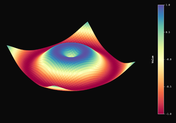
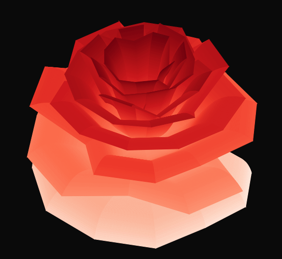
![]() Parametric surface support
Parametric surface support
Free and open source code is here:
Simply download the folder, install bokeh numpy pandas and xarray, and run the python EXAMPLE*.py.
Simple example:
from surface3d_py import Surface3D
from bokeh.plotting import show, output_file
import numpy as np

x = np.linspace(-5, 5, 50)
y = np.linspace(-5, 5, 50)
X, Y = np.meshgrid(x, y)
Z = np.sin(np.sqrt(X**2 + Y**2))

surf = Surface3D(
    lons=X.flatten().tolist(),
    lats=Y.flatten().tolist(),
    values=Z.flatten().tolist(),
    n_lat=50,
    n_lon=50,
    palette='Spectral',
    autorotate=True,
)
show(surf)
Further examples included in the above folder:

import numpy as np
from surface3d_py import Surface3D
from bokeh.plotting import show, output_file

# Parameters
n_lat, n_lon = 70, 70
u = np.linspace(0, 2*np.pi, n_lon)  # angular param
v = np.linspace(0, np.pi, n_lat)    # vertical param
U, V = np.meshgrid(u, v)

# Julia's parametric heart surface
X = np.sin(V) * (15 * np.sin(U) - 4 * np.sin(3*U))
Y = 8 * np.cos(V)
Z = np.sin(V) * (15 * np.cos(U) - 5 * np.cos(2*U) - 2 * np.cos(3*U) - np.cos(4*U))

# Flatten for Surface3D
lons = X.flatten()
lats = Z.flatten()   # swap Z to lat so rotation looks better
values = Y.flatten()  # Y as height

# Create Surface3D
surface = Surface3D(
    lons=lons.tolist(),
    lats=lats.tolist(),
    values=values.tolist(),
    n_lat=n_lat,
    n_lon=n_lon,
    palette='Reds_r',
    autorotate=True,
    zoom=0.8,
    width=800,
    height=800,
    background_color='#0a0a0a',
    colorbar_text_color='#ffffff',
    show_colorbar=False,
    elevation=60,
    azimuth=-30,
)

output_file("julia_heart.html")
show(surface)
import numpy as np
import math

# Helper functions
def square(x):
    return x * x

def mod2(a, b):
    c = a % b
    return c if c > 0 else c + b

# Create sample data - a parametric rose surface
n_lat, n_lon = 100, 100  # u_steps, v_steps in parametric terms

# Parameter ranges
u = np.linspace(0, 1, n_lat)  # x1 parameter
v = np.linspace(-(20/9)*math.pi, 15*math.pi, n_lon)  # theta parameter

# Create meshgrids
u_grid, v_grid = np.meshgrid(u, v)

# Initialize arrays for coordinates
x = np.zeros_like(u_grid)
y = np.zeros_like(u_grid)
z = np.zeros_like(u_grid)

# Calculate parametric rose surface
for i in range(n_lon):
    for j in range(n_lat):
        theta = v[i]
        x1 = u[j]

        # Calculate phi
        phi = (math.pi / 2) * math.exp(-theta / (8 * math.pi))

        # Calculate y1
        y1 = (1.9565284531299512 * square(x1) *
              square(1.2768869870150188 * x1 - 1) * math.sin(phi))

        # Calculate X
        X = 1 - square(1.25 * square(1 - mod2(3.6 * theta, 2 * math.pi) / math.pi) - 0.25) / 2

        # Calculate r
        r = X * (x1 * math.sin(phi) + y1 * math.cos(phi))

        # Calculate coordinates (centered at origin)
        x[i, j] = r * math.sin(theta)
        y[i, j] = r * math.cos(theta)
        z[i, j] = X * (x1 * math.cos(phi) - y1 * math.sin(phi))

# Use x and y as lat/lon equivalents, z as values
lon_grid = x
lat_grid = y
values = z

# Flatten for the component
lons_flat = lon_grid.flatten()
lats_flat = lat_grid.flatten()
values_flat = values.flatten()
# Create the Surface3D visualization with colorbar
surface = Surface3D(
    lons=lons_flat.tolist(),
    lats=lats_flat.tolist(),
    values=values_flat.tolist(),
    n_lat=n_lat,
    n_lon=n_lon,
    width=800,
    height=800,
    palette='Reds',
    azimuth=45,
    elevation=-40,
    zoom=1.0,
    autorotate=True,
    rotation_speed=1.0,
    enable_hover=True,
    # Colorbar properties
    show_colorbar=True,
    colorbar_title='Surface Value',
    # Appearance
    background_color='#0a0a0a',
    colorbar_text_color='#ffffff'
)

show(surface)
from surface3d_py import Surface3D
from bokeh.plotting import show, output_file
import numpy as np
import xarray as xr
import numpy as np
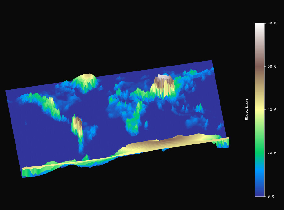
# Load and coarsen
ds = xr.open_dataset("elev.nc")
ds_coarse = ds.coarsen(latitude=5, longitude=5, boundary='trim').mean()
# Choose the variable (check ds_coarse)
elev = ds_coarse["elevation"]
# Flip latitude if needed
# elev = elev.isel(latitude=slice(None, None, -1))
# elev = elev.isel(longitude=slice(None, None, -1))
# Get coarsened dimensions
n_lat, n_lon = elev.shape
lons = elev.longitude.values
lats = elev.latitude.values
Zraw = elev.values
# Normalize
Znorm = (Zraw - np.nanmean(Zraw)) / np.nanstd(Zraw)
Znorm = 80 * (Zraw - np.nanmin(Zraw)) / (np.nanmax(Zraw) - np.nanmin(Zraw))
# Flatten in row-major order (first lat, then lon)
lons_flat, lats_flat = np.meshgrid(lons, lats)
lons_flat = lons_flat.flatten()
lats_flat = lats_flat.flatten()
values_flat = Znorm.flatten()
print(f"n_lat={n_lat}, n_lon={n_lon}, len(values_flat)={len(values_flat)}")
surface = Surface3D(
lons=lons_flat.tolist(),
lats=lats_flat.tolist(),
values=values_flat.tolist(),
n_lat=n_lat,
n_lon=n_lon,
width=800,
height=800,
palette='terrain',
azimuth=45,
elevation=-30,
zoom=1.0,
autorotate=False,
rotation_speed=1.0,
enable_hover=True,
show_colorbar=True,
colorbar_title='Elevation',
background_color='#0a0a0a',
colorbar_text_color='#ffffff'
)
show(surface)

# Parameters
n_lat, n_lon = 100, 100
u = np.linspace(0, 2*np.pi, n_lon)   # angular
v = np.linspace(0, 1, n_lat)         # height / radius scaling
U, V = np.meshgrid(u, v)
# Helix shape with radius oscillations
x = (1 + 0.3*np.sin(5*V*np.pi)) * np.cos(4*np.pi*V)
y = (1 + 0.3*np.sin(5*V*np.pi)) * np.sin(4*np.pi*V)
z = 5*V + 0.2*np.sin(10*U)

lons = x.flatten()
lats = y.flatten()
values = z.flatten()

surface = Surface3D(
    lons=lons.tolist(),
    lats=lats.tolist(),
    values=values.tolist(),
    n_lat=n_lat,
    n_lon=n_lon,
    palette='cool',
    autorotate=True,
    zoom=1.0,
    background_color='#0a0a0a',
    colorbar_text_color='#ffffff'
)

output_file("vine.html")
show(surface)
import numpy as np
from bokeh.plotting import show, output_file
from surface3d_py import Surface3D
# Your plotting function
def plot_surface_bokeh(func, title="Surface", output_path="surface.html", n_lat=100, n_lon=100):
# Create grid
x = np.linspace(-5, 5, n_lon)
y = np.linspace(-5, 5, n_lat)
X, Y = np.meshgrid(x, y)
# Compute Z
Z = func(X, Y)
# Flatten for Surface3D
lons = X.flatten()
lats = Y.flatten()
values = Z.flatten()
surface = Surface3D(
lons=lons.tolist(),
lats=lats.tolist(),
values=values.tolist(),
n_lat=n_lat,
n_lon=n_lon,
palette='Spectral',
autorotate=True,
zoom=0.8,
width=800,
height=800,
background_color='#0a0a0a',
colorbar_text_color='#ffffff',
show_colorbar=True
)
output_file(output_path, title=title)
return surface
# List of surfaces
best_surfaces = [
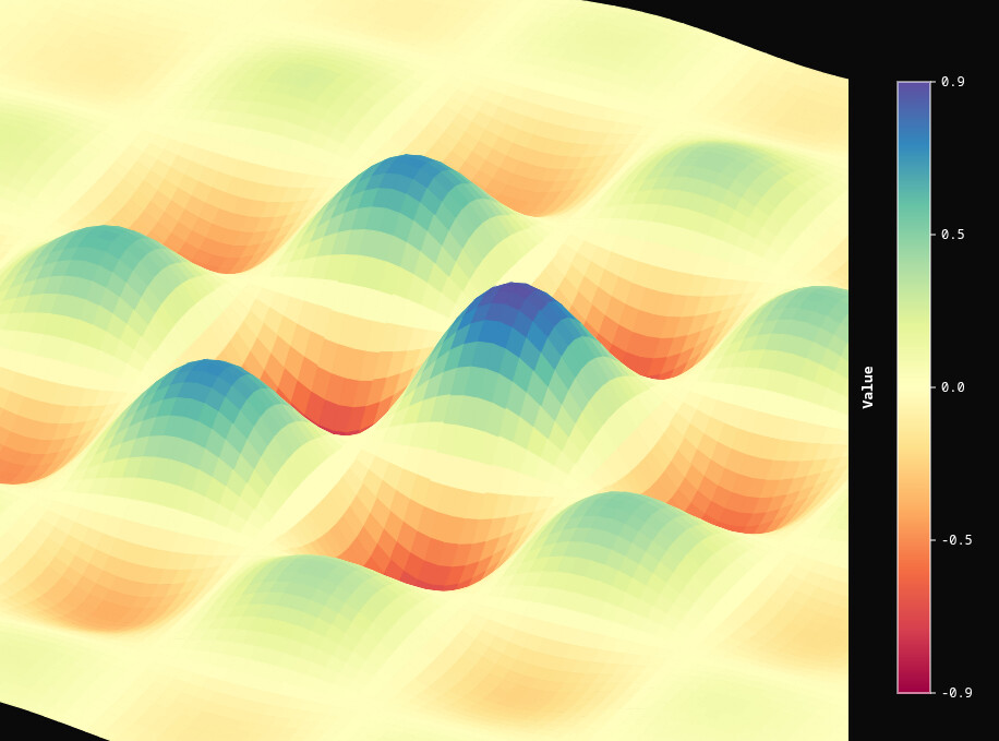
(lambda X,Y: np.sin(X*2) * np.cos(Y*2), "Smooth Wave Hills"),
(lambda X,Y: np.sin(3*np.sqrt(X**2 + Y**2))/np.sqrt(X**2 + Y**2 + 1e-6), "Circular Ripple"),
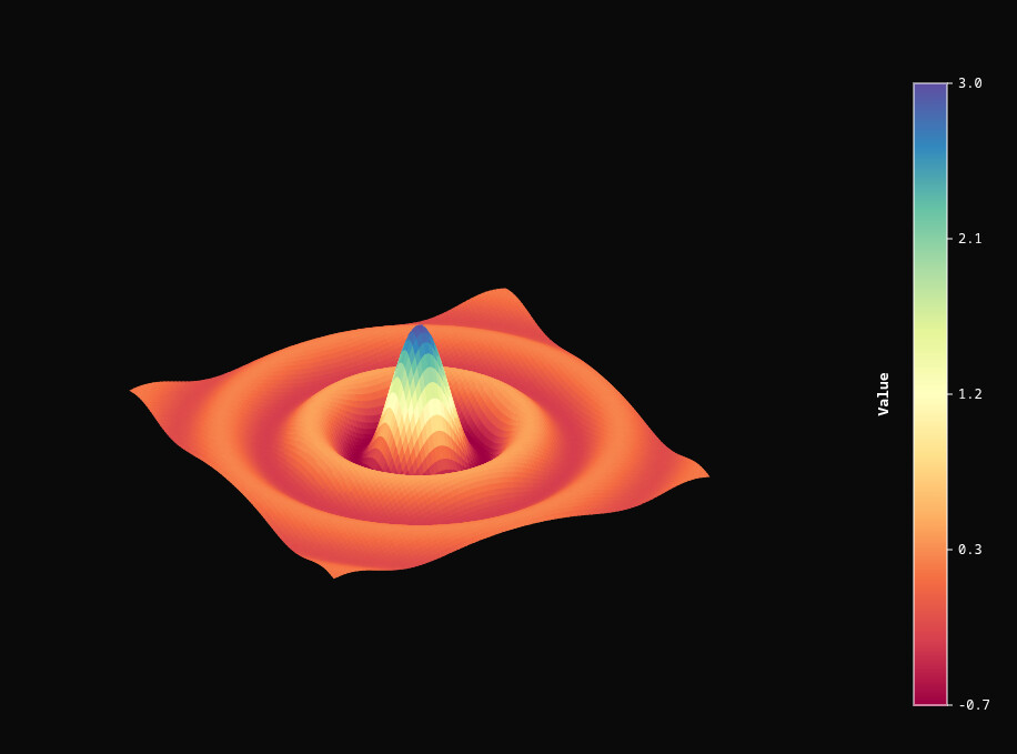
(lambda X,Y: (1 - (X**2 + Y**2)) * np.exp(-(X**2 + Y**2)/2), "Mexican Hat"),
(lambda X,Y: np.sin(X)*np.cos(Y), "sin(X)*cos(Y)"),
(lambda X,Y: np.sin(np.sqrt(X**2 + Y**2)), "sin(sqrt(X^2+Y^2))"),
(lambda X,Y: np.exp(-0.1*(X**2+Y**2))*np.sin(X*2)*np.cos(Y*2), "damped sine-cosine"),
(lambda X,Y: np.tanh(X)*np.tanh(Y), "tanh(X)*tanh(Y)"),
(lambda X,Y: np.sin(X)*np.sin(Y) + np.cos(X*Y), "sin(X)*sin(Y)+cos(X*Y)")
]
# Loop through and plot
for idx, (func, name) in enumerate(best_surfaces, 1):
plot = plot_surface_bokeh(func, title=f"Surface {idx}: {name}", output_path=f"surface_best_{idx}.html")
show(plot)