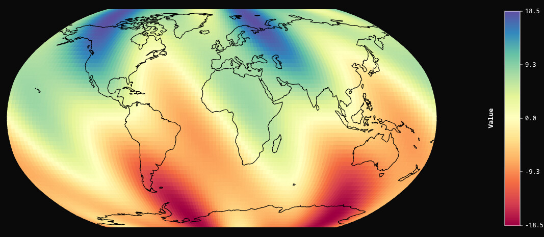
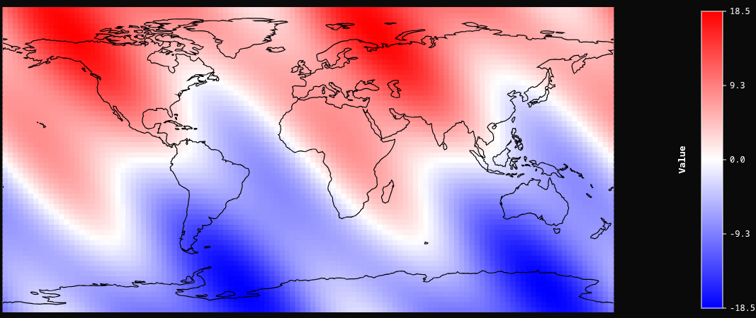
A custom BokehJS extension that visualizes gridded data on flat map projections. Supports several projections including Mercator, Robinson, Mollweide, Natural Earth, Winkel Tripel, and Albers Equal Area. Pan with drag, zoom with scroll, and rotate the map horizontally. Auto-loads Natural Earth coastlines and country borders. Great for climate data, ocean currents, atmospheric patterns, or any global dataset that works better on flat maps than globes.
Free and open source code is here:
Simply download the folder, install bokeh numpy pandas and xarray (no need for cartopy!), and run the several examples.
Simple example:
########### mollweide ###########
from gridded_projection_py import GriddedProjection
from bokeh.plotting import show
import numpy as np

lons = np.linspace(-180, 180, 120)
lats = np.linspace(-90, 90, 60)
lons_grid, lats_grid = np.meshgrid(lons, lats)
values = ( 10 * np.sin(np.radians(lats_grid)) + 6  * np.sin(2 * np.radians(lons_grid)) + 3  * np.sin(4 * np.radians(lats_grid + lons_grid)) )

proj = GriddedProjection(
    lons=lons_grid.flatten().tolist(),
    lats=lats_grid.flatten().tolist(),
    values=values.flatten().tolist(),
    n_lat=60,
    n_lon=120,
    projection='mollweide',
    palette='terrain',
)
show(proj)

Interactive Explorer with CustomJS:
"""
Interactive GriddedProjection Dashboard
========================================
Pure-Bokeh, no server required. All controls are wired through CustomJS
callbacks so every change updates the map instantly in the browser.
Requirements
------------
* bokeh
* numpy
* The GriddedProjection custom model (gridded_projection_py.py + the
compiled gridded_projection.ts) must be importable from the same directory.
Run
---
python dashboard.py
"""
import numpy as np
from bokeh.plotting import save, show, output_file
from bokeh.layouts import column, row
from bokeh.models import (
Dropdown, Select, CheckboxGroup, ColorPicker,
CustomJS, Div, Spacer, Label
)
from bokeh.core.serialization import Serializer # only used for type hint; safe to skip
from gridded_projection_py import GriddedProjection
# ═══════════════════════════════════════════════════════════════════════════════
# 1. DATA SAMPLES – four "natural-looking" global fields
# ═══════════════════════════════════════════════════════════════════════════════
N_LON, N_LAT = 180, 90 # grid resolution (lon × lat)
_lons1d = np.linspace(-180, 180, N_LON)
_lats1d = np.linspace(-90, 90, N_LAT)
_LON, _LAT = np.meshgrid(_lons1d, _lats1d)
_lon_r, _lat_r = np.radians(_LON), np.radians(_LAT)
def _sample_temperature():
"""
Synthetic global surface-temperature-like field.
Warm tropics, cold poles, slight land-sea contrast via a cosine bump.
"""
base = 15.0 - 40.0 * (_lat_r ** 2) / (np.pi / 2) ** 2 # parabolic pole cooling
land = 5.0 * np.cos(2.5 * _lon_r) * np.cos(1.8 * _lat_r) # zonal "continent" warmth
noise = 2.0 * np.sin(7 * _lon_r) * np.sin(5 * _lat_r) # small-scale texture
return base + land + noise
def _sample_pressure():
"""
Synthetic sea-level-pressure-like field.
Alternating high/low centres reminiscent of the subtropical highs and
polar lows, with a slight hemispheric asymmetry.
"""
# Three subtropical high centres (roughly correct positions)
highs = (
1013 + 18 * np.exp(-(((_lon_r - np.radians(-30))**2) / 0.4 + ((_lat_r - np.radians(30))**2) / 0.25))
+ 15 * np.exp(-(((_lon_r - np.radians(130))**2) / 0.5 + ((_lat_r - np.radians(25))**2) / 0.22))
+ 14 * np.exp(-(((_lon_r - np.radians(-120))**2) / 0.45 + ((_lat_r - np.radians(28))**2) / 0.24))
)
# Polar low influence
polar = -12 * np.exp(-((_lat_r - np.radians(55))**2) / 0.18)
polar -= 10 * np.exp(-((_lat_r + np.radians(60))**2) / 0.20)
# Equatorial low band (ITCZ-ish)
itcz = -6 * np.exp(-(_lat_r**2) / 0.04)
return highs + polar + itcz
def _sample_wind_speed():
"""
Synthetic global wind-speed field.
Jet streams at ~±35° lat, trade-wind bands in the tropics, calm subtropics.
"""
# Jet streams (narrow bands of high wind)
jets = (12 * np.exp(-((_lat_r - np.radians(38))**2) / 0.03)
+ 10 * np.exp(-((_lat_r + np.radians(42))**2) / 0.035))
# Trade winds (broader, lower)
trades = 7 * np.cos(_lon_r * 0.5) * np.exp(-((_lat_r)**2) / 0.12)
# Calm subtropics (dip)
calm = -4 * (np.exp(-((_lat_r - np.radians(25))**2) / 0.06)
+ np.exp(-((_lat_r + np.radians(25))**2) / 0.06))
# Polar westerlies
westerlies = 6 * np.exp(-((_lat_r - np.radians(55))**2) / 0.08) * (1 + 0.3 * np.sin(2 * _lon_r))
return np.clip(jets + trades + calm + westerlies + 3, 0, None) # speed ≥ 0
def _sample_ocean_depth():
"""
Synthetic bathymetry / elevation field.
Deep ocean basins, mid-ocean ridges along ~0° and ~180° lon, shallow
continental shelves near the "land" longitudes, and mountain ranges.
"""
# Ocean basins (deep negative)
pac = -4500 * np.exp(-(((_lon_r - np.radians(170))**2) / 1.2 + ((_lat_r)**2) / 0.8))
atl = -3800 * np.exp(-(((_lon_r - np.radians(-35))**2) / 0.6 + ((_lat_r)**2) / 1.0))
ind = -3200 * np.exp(-(((_lon_r - np.radians(80))**2) / 0.5 + ((_lat_r + np.radians(15))**2) / 0.4))
# Mid-ocean ridges (shallower lines through basins)
ridge = 1800 * np.exp(-((np.abs(_lon_r - np.radians(-30)) - 0.05)**2) / 0.01) * np.exp(-(_lat_r**2)/2.0)
# Continental shelves / land masses (positive near "continents")
land = 2000 * np.exp(-(((_lon_r - np.radians(30))**2) / 0.3 + ((_lat_r - np.radians(40))**2) / 0.35))
land += 1800 * np.exp(-(((_lon_r - np.radians(-100))**2) / 0.4 + ((_lat_r - np.radians(35))**2) / 0.3))
land += 1500 * np.exp(-(((_lon_r - np.radians(110))**2) / 0.35 + ((_lat_r - np.radians(20))**2) / 0.25))
# Mountain peaks
mtn = 3500 * np.exp(-(((np.radians(_LON) - np.radians(75))**2) / 0.02 + ((_lat_r - np.radians(32))**2) / 0.01)) # Himalayas-ish
return pac + atl + ind + ridge + land + mtn
SAMPLES = {
"Sample 1 – Temperature (°C)": _sample_temperature(),
"Sample 2 – Pressure (hPa)": _sample_pressure(),
"Sample 3 – Wind Speed (m/s)": _sample_wind_speed(),
"Sample 4 – Bathymetry (m)": _sample_ocean_depth(),
}
# Flatten lons/lats once; value arrays are built per-sample below.
FLAT_LONS = _LON.flatten().tolist()
FLAT_LATS = _LAT.flatten().tolist()
# ═══════════════════════════════════════════════════════════════════════════════
# 2. WIDGET DEFINITIONS
# ═══════════════════════════════════════════════════════════════════════════════
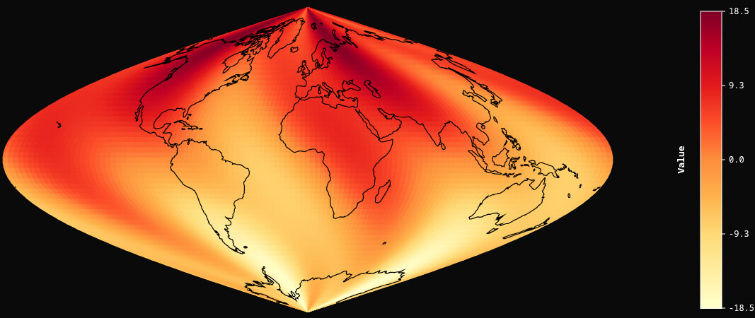
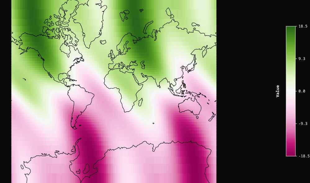
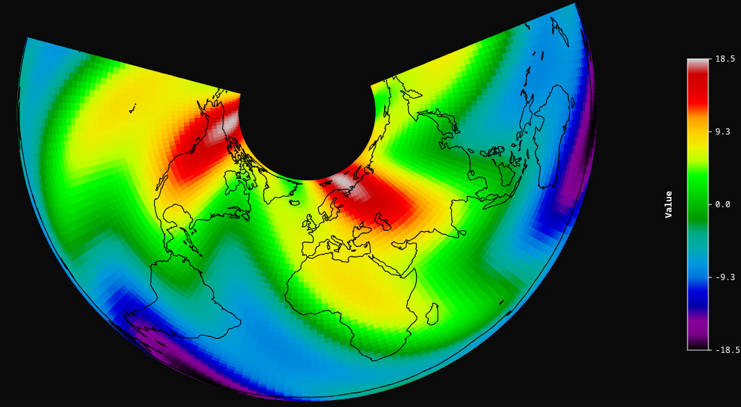
PROJECTIONS = [ "natural_earth", "mollweide", "robinson", "plate_carree", "sinusoidal", "eckert4", "winkel_tripel", "miller", "mercator", "albers_equal_area", ]
PALETTES = [ "Turbo256", "Viridis256", "Plasma256", "Inferno256", "Magma256", "Cividis256", "terrain", "YlOrRd", "RdYlBu", "bwr", "Spectral", "RdYlGn", "PiYG", "BuPu", "nipy_spectral", "coolwarm","cool","seismic","winter","summer","autumn","spring", "rainbow","gist_earth" ]
projection_select = Select( title="Projection", value="robinson", options=PROJECTIONS, width=220, styles={"font-size": "13px"} )
palette_select = Select( title="Palette", value="Spectral", options=PALETTES, width=220, styles={"font-size": "13px"} )
data_select = Select( title="Data Sample", value="0", options=[(str(i), name) for i, name in enumerate(SAMPLES.keys())], width=220, styles={"font-size": "13px"} )
# Checkboxes: 0 = coastlines, 1 = countries
overlay_checkboxes = CheckboxGroup( labels=["Show Coastlines", "Show Countries"], active=[0,1], styles={"font-size": "13px"} )
coastline_picker = ColorPicker( title="Coastline Color", color="#000000", width=70, styles={"font-size": "13px"} )
country_picker = ColorPicker( title="Country Border Color", color="#000000", width=70, styles={"font-size": "13px"} )
# ═══════════════════════════════════════════════════════════════════════════════
# 3. THE MAP MODEL (created once; JS mutates its properties)
# ═══════════════════════════════════════════════════════════════════════════════
SAMPLE_NAMES = list(SAMPLES.keys()) # ["Sample 1 – …", …]
SAMPLE_VALUES = [SAMPLES[k].flatten().tolist() for k in SAMPLE_NAMES] # list of flat arrays
map_model = GriddedProjection(
lons=FLAT_LONS,
lats=FLAT_LATS,
values=SAMPLE_VALUES[0],
n_lat=N_LAT,
n_lon=N_LON,
projection="robinson",
palette="Spectral",
show_coastlines=True,
coastline_color="#000000",
coastline_width=0.6,
show_countries=True,
country_color="#000000",
country_width=0.5,
background_color="#f0f0f0",
colorbar_text_color="#494949",
colorbar_title="Value",
width=900,
height=520,
)
# Park all value arrays on .tags so JS can reach them as map_model.tags[i]
# (same technique the sphere example uses)
map_model.tags = SAMPLE_VALUES
# ═══════════════════════════════════════════════════════════════════════════════
# 4. CUSTOM JS – one shared callback, attached to every widget
# ═══════════════════════════════════════════════════════════════════════════════
JS_CODE = """
(function() {
// All names here are injected bare by Bokeh — no "args." prefix.
var idx = parseInt(data_select.value);
var newVals = gmap.tags[idx];
gmap.projection = projection_select.value;
gmap.palette = palette_select.value;
gmap.values = newVals;
gmap.colorbar_title = sample_names[idx];
gmap.show_coastlines = overlay_checkboxes.active.indexOf(0) !== -1;
gmap.show_countries = overlay_checkboxes.active.indexOf(1) !== -1;
gmap.coastline_color = coastline_picker.color;
gmap.country_color = country_picker.color;
})();
"""
shared_cb = CustomJS(args=dict(
gmap=map_model,
projection_select=projection_select,
palette_select=palette_select,
data_select=data_select,
overlay_checkboxes=overlay_checkboxes,
coastline_picker=coastline_picker,
country_picker=country_picker,
sample_names=SAMPLE_NAMES, # plain list of strings, easy to serialise
), code=JS_CODE)
# Attach to every widget that should trigger an update
projection_select.js_on_change("value", shared_cb)
palette_select.js_on_change("value", shared_cb)
data_select.js_on_change("value", shared_cb)
overlay_checkboxes.js_on_change("active", shared_cb)
coastline_picker.js_on_change("color", shared_cb)
country_picker.js_on_change("color", shared_cb)
# ═══════════════════════════════════════════════════════════════════════════════
# 5. LAYOUT & OUTPUT
# ═══════════════════════════════════════════════════════════════════════════════
title_div = Div(text="""
<div style="
background: linear-gradient(135deg, #dbdbdb 0%, #faa4a4 100%);
border-radius: 12px 12px 0 0;
padding: 18px 28px;
border-bottom: 1px solid #faa4a4;
">
<h2 style="margin:0; color:#0f0f0f; font-weight:600; font-size:20px; letter-spacing:0.3px;">
🌍 Global Projection Explorer
</h2>
<p style="margin:6px 0 0; color:#000000; font-size:13px; font-weight:400;">
Switch projections, palettes and data fields instantly.
</p>
</div>
""", width=400)
layout = row(
column(
title_div,
projection_select,palette_select,data_select, overlay_checkboxes,coastline_picker,country_picker,),
map_model, styles = {"border": "1px solid #faa4a4", "border-radius": "12px","background": "#f0f0f0", "width": "1500px"}
)
show(layout)
Interactive Animation with CustomJS (really fast animation):
"""
Animated GriddedProjection - CustomJS Version
==============================================
12 years of gridded data with time slider and play button.
Pure client-side JavaScript - no server required.

Run with: python animated_gridded_customjs.py
"""

import numpy as np
from bokeh.plotting import show
from bokeh.layouts import column, row
from bokeh.models import Slider, Button, Div, CustomJS
from gridded_projection_py import GriddedProjection

# ═══════════════════════════════════════════════════════════════════════════════
# 1. GENERATE 12 YEARS OF DATA
# ═══════════════════════════════════════════════════════════════════════════════

N_YEARS = 12
lons = np.linspace(-180, 180, 120)
lats = np.linspace(-90, 90, 60)
lons_grid, lats_grid = np.meshgrid(lons, lats)

# Generate data for each year with evolving patterns
yearly_data = []
for year in range(N_YEARS):
    # Base pattern with time evolution
    time_factor = year / N_YEARS * 2 * np.pi

    values = (
        10 * np.sin(np.radians(lats_grid)) +
        6 * np.sin(2 * np.radians(lons_grid) + time_factor) +
        3 * np.sin(4 * np.radians(lats_grid + lons_grid) + time_factor * 0.5) +
        2 * np.cos(np.radians(lons_grid) * 3 - time_factor)
    )
    yearly_data.append(values.flatten().tolist())

# ═══════════════════════════════════════════════════════════════════════════════
# 2. CREATE MAP MODEL
# ═══════════════════════════════════════════════════════════════════════════════

proj = GriddedProjection(
    lons=lons_grid.flatten().tolist(),
    lats=lats_grid.flatten().tolist(),
    values=yearly_data[0],  # Start with year 0
    n_lat=60,
    n_lon=120,
    projection='robinson',
    palette='Spectral',
    colorbar_title='Year 2013',
    width=900,
    height=500,
        background_color="#f0f0f0",
    colorbar_text_color="#333333",
)

# Store all yearly data in the model's tags for JS access
proj.tags = yearly_data

# ═══════════════════════════════════════════════════════════════════════════════
# 3. CREATE WIDGETS
# ═══════════════════════════════════════════════════════════════════════════════

year_slider = Slider(
    start=0,
    end=N_YEARS - 1,
    value=0,
    step=1,
    title="Year",
    width=700,
    bar_color="#ff6b6b",

)

play_button = Button(
    label="▶ Play",
    button_type="success",
    width=100,
)

title_div = Div(text="""
<div style="
    background: linear-gradient(135deg, #667eea 0%, #764ba2 100%);
    border-radius: 8px;
    padding: 16px 24px;
    margin-bottom: 15px;
">
    <h2 style="margin:0; color:white; font-weight:600; font-size:22px;">
        🌍 Climate Data Animation (2013-2024)
    </h2>
    <p style="margin:6px 0 0; color:#f0f0f0; font-size:14px;">
        Use the slider or play button to animate through 12 years of data
    </p>
</div>
""", width=900)

# ═══════════════════════════════════════════════════════════════════════════════
# 4. CUSTOMJS CALLBACKS
# ═══════════════════════════════════════════════════════════════════════════════

# Slider callback: update map when slider changes
slider_callback = CustomJS(args=dict(proj=proj, slider=year_slider), code="""
    const year_idx = Math.round(slider.value);
    const year_label = 2013 + year_idx;

    // Update map data from stored tags
    proj.values = proj.tags[year_idx];
    proj.colorbar_title = 'Year ' + year_label;

""")

year_slider.js_on_change('value', slider_callback)

# Play button callback: start/stop animation
play_callback = CustomJS(args=dict(
    slider=year_slider,
    button=play_button,
    proj=proj,
    n_years=N_YEARS
), code="""
    // Animation interval stored on button itself
    if (button.interval_id === undefined) {
        button.interval_id = null;
        button.is_playing = false;
    }

    if (button.is_playing) {
        // Stop animation
        if (button.interval_id !== null) {
            clearInterval(button.interval_id);
            button.interval_id = null;
        }
        button.label = "▶ Play";
        button.button_type = "success";
        button.is_playing = false;
    } else {
        // Start animation
        button.interval_id = setInterval(function() {
            let new_year = slider.value + 1;
            if (new_year >= n_years) {
                new_year = 0;
            }
            slider.value = new_year;

            // Update map directly (slider callback will also fire)
            const year_idx = Math.round(new_year);
            const year_label = 2013 + year_idx;
            proj.values = proj.tags[year_idx];
            proj.colorbar_title = 'Year ' + year_label;

        }, 500);  // 500ms = 0.5 sec per year

        button.label = "⏸ Pause";
        button.button_type = "warning";
        button.is_playing = true;
    }
""")

play_button.js_on_click(play_callback)

# ═══════════════════════════════════════════════════════════════════════════════
# 5. LAYOUT
# ═══════════════════════════════════════════════════════════════════════════════

controls = row(play_button, year_slider, spacing=10)

layout = column(
    title_div,
    controls,
    proj,
    sizing_mode='fixed',styles = {"border": "1px solid #faa4a4", "border-radius": "12px","background": "#f0f0f0", "width": "1100px", "height": "700px"}
)

show(layout)