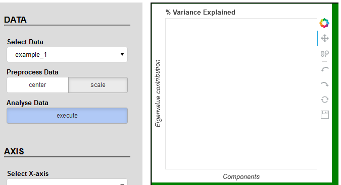
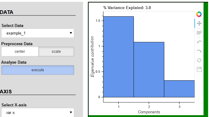
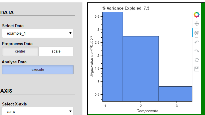
I was trying to find the solution but without success. Please check the code and play with buttons and tools. I’m still facing same problems with plot_1 as described in points 2 and 3. According to the console data has correct values.
index.html
<!DOCTYPE html>
<html lang="en">
  <head>
    <meta charset="utf-8">
    {{ bokeh_css }}
    {{ bokeh_js }}
    <link rel="stylesheet" href="bokeh/static/css/style.css"/>
  </head>
  <body>


{% extends base %}
{% block contents %}

<div class='grid'>
    <div class='panel'>
        <p class='axs'>DATA</p><hr><br />
        {{ embed(roots.menu_dataset) }}

    </div>
    <div class='plot_1'>{{ embed(roots.plot_1) }}</div>
    <div class='plot_2'>{{ embed(roots.plot_2) }}</div>
</div>

{% endblock %}
</body>
</html>
main.py
import numpy as np
np.set_printoptions(precision=4, suppress=True)
import pandas as pd
from bokeh.io import curdoc
from bokeh.models import FactorRange, DataRange1d, ColumnDataSource
from bokeh.models import Select, Button, RadioButtonGroup, Column, Div, HoverTool, Span
from bokeh.plotting import figure
#--> data loading
def load_data(database):
if database == 'example_1':
a = [1,2,3]
b = [2,4,2]
c = [3,2,5]
d = [4,5,1]
e = [5,1,2]
data = np.vstack((a,b,c,d,e))
elif database == 'example_2':
a = [1,3,1]
b = [4,4,3]
c = [2,2,2]
d = [3,2,4]
e = [5,5,0]
f = [60,2,3]
data = np.vstack((a,b,c,d,e,f))
return data
#--> data preprocessing
def preprocess_data(data, standardize):
mu = np.mean(data, axis=0)
data_cen = data - mu
data_std = data_cen / np.std(data, axis=0, ddof=1)
if standardize == 'center':
return data_cen
elif standardize == 'scale':
return data_std
#--> decomposition
def SVD_decompose(data):
L = data.T@data
return L
def initialize():
# data setting
data = load_data(select_data.value)
standardize = preprocess_[btng_norm.active]
X = preprocess_data(data, standardize)
n = X.shape[0]
p = X.shape[1]
component = ['#' + str(i) for i in range(1, p+1)]
L = SVD_decompose(X)
# CDS
CDS_lambda.data.update({'component': component,
'lambda': np.diag(L),
'proportion': np.diag(L)/L.trace(),
'cumsum_proportion': np.cumsum(np.diag(L)/L.trace())})
# ranges
x_.update(factors = component,
bounds = (0, len(component)))
y_1.update(start = 0,
end = 1.05*np.diag(L).max(),
bounds = (0, 1.05*np.diag(L).max()))
examples_ = ['example_1', 'example_2'] #--> example_1
preprocess_ = ['center', 'scale'] #--> scale
select_data = Select(title = 'Select Data', value = examples_[0], options = examples_)
btng_norm = RadioButtonGroup(labels = preprocess_, active = 1, margin=(0, 5, 5, 5))
btn_run = Button(label='execute', css_classes=['pad', 'btn_style'], margin=(0, 5, 5, 5))
data_lambda = {'component': [],
'lambda': [],
'proportion': [],
'cumsum_proportion': []}
CDS_lambda = ColumnDataSource(data=data_lambda)
x_ = FactorRange()
y_1 = DataRange1d()
y_2 = DataRange1d(start=0, end=1.05, bounds=(0, 1.05))
initialize()
print(CDS_lambda.data)
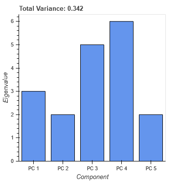
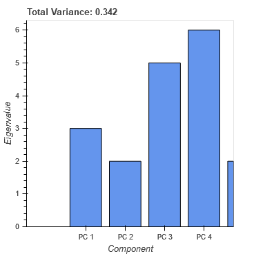
# plot_1
plot_1 = figure(frame_width=300, frame_height=300, match_aspect=False,
x_range=x_, y_range=y_1,
name='plot_1')
plot_1.title.text = 'Total Variance: {:0.3f}'.format(CDS_lambda.data['lambda'].sum())
plot_1.xaxis.axis_label = 'Components'
plot_1.yaxis.axis_label = 'Eigenvalue contribution'
plot_1.xgrid.visible = None
plot_1.ygrid.visible = None
bar = plot_1.vbar(x='component', top='lambda', source=CDS_lambda, width=1)
avg = plot_1.add_layout(Span(location=CDS_lambda.data['lambda'].mean()))
hover_lambda = HoverTool(
tooltips=[('PC', '@component'),
(chr(955), '@lambda{0.000}')],
mode='mouse')
hover_lambda.renderers=[bar]
plot_1.add_tools(hover_lambda)
# plot_2
plot_2 = figure(frame_width=300, frame_height=300, match_aspect=False,
x_range=x_, y_range=y_2,
name='plot_2')
plot_2.title.text = '% Variance Explained'
plot_2.xaxis.axis_label = 'Components'
plot_2.yaxis.axis_label = 'Eigenvalue contribution'
plot_2.xgrid.visible = None
plot_2.ygrid.visible = True
#plot_2.legend.location = (180,30)
#plot_2.legend.click_policy='hide'
plot_2.line(x='component', y='proportion', source=CDS_lambda, line_color='blue', legend_label='proportion')
pro = plot_2.circle(x='component', y='proportion', source=CDS_lambda, line_color='blue', legend_label='proportion', size=7, fill_color='white', hover_fill_color='red')
plot_2.line(x='component', y='cumsum_proportion', source=CDS_lambda, line_color='black', legend_label='cumulative')
cum = plot_2.circle(x='component', y='cumsum_proportion', source=CDS_lambda, line_color='black', legend_label='cumulative', size=7, fill_color='white', hover_fill_color='red')
hover_variance = HoverTool(
tooltips=[('PC', '@component'),
('proportion', '@proportion{0.000}'),
('cumulative', '@cumsum_proportion{0.000}')],
mode='vline')
hover_variance.renderers=[pro, cum]
plot_2.add_tools(hover_variance)
def execute():
data = load_data(select_data.value)
standardize = preprocess_[btng_norm.active]
X = preprocess_data(data, standardize)
n = X.shape[0]
p = X.shape[1]
component = ['#' + str(i) for i in range(1, p+1)]
L = SVD_decompose(X)
# CDS
CDS_lambda.data.update({'component': component,
'lambda': np.diag(L),
'proportion': np.diag(L)/L.trace(),
'cumsum_proportion': np.cumsum(np.diag(L)/L.trace())})
x_.update(factors = component,
bounds = (0, len(component)))
y_1.update(start = 0,
end = 1.05*np.diag(L).max(),
bounds = (0, 1.05*np.diag(L).max()))
plot_1.title.text = '% Variance Explaied: {:0.3f}'.format(np.diag(L).sum())
print()
print(CDS_lambda.data)
print(x_.bounds)
print(y_1.bounds)
print(y_1.start)
print(y_1.end)
print()
btn_run.on_click(execute)
print(x_.bounds)
print(y_1.bounds)
print(y_1.start)
print(y_1.end)
print()
#--> sidebar
menu_dataset = Column(select_data, Div(text="""Preprocess Data""", margin=(5, 5, 0, 5), css_classes=['missing_labels']),
btng_norm, Div(text="""Analyse Data""", margin=(5, 5, 0, 5), css_classes=['missing_labels']),
btn_run, name='menu_dataset', width=250)
curdoc().add_root(menu_dataset)
curdoc().add_root(plot_1)
curdoc().add_root(plot_2)
curdoc().title = "My dashboard"