cProfiling vanilla Bokeh vs GeoViews+Bokeh vs hvPlot+Bokeh

I’m currently comparing different Python visualisation libraries for a thesis, including different interfaces to Bokeh. One part is comparing the total CPU runtimes of each library to generate the same map product using the same data. The performance benchmarking is done with cProfile.

The basic setup is this: After the data has been prepared and transformed to where each of the libraries can handle it directly (the prepGDFs() function), I’m wrapping all figure and axes definitions, including the central call to bokeh.plotting.figure, in a function called renderFigure() which is then wrapped with a decorator that basically does this:

p = cProfile.Profile() 
p.enable() # start cProfiling

value = func(*args, **kwargs) # execute renderFigure()

p.disable() # stop cProfiling
p.dump_stats() # write cProfile to file

Due to different libraries employing different rendering strategies, I decided to try and force each of them to render the figure in VSCode rather than, say, some in VSCode and some in a browser window. To achieve this, a few adjustments were made to each of the libraries (see the table under point 5 of the ‘How are libraries being compared?’ section which Discourse won’t let me link to as a new user…). For Bokeh, this meant adding

bokeh.io.output.output_notebook()
…
bokeh.io.show(plot)

Now, the results are currently quite favorable to the vanilla Bokeh interface, as you can see below for the rendering of a large 144,000 polygon dataset.

comp_profile_interactive_dd

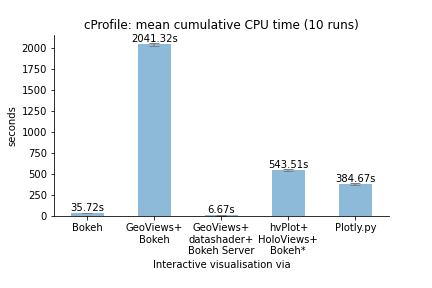
The only puzzling thing is this: vanilla Bokeh’s mean CPU runtime measured by cProfile seems to differ substantially from when the figure is in fact rendered in the VSCode interpreter: I manually observed (basically, stopwatched) the time between the completion of the prior prepGDFs() function completing and the plot being fully rendered to be around 125 seconds instead of the roughly 35 seconds recorded by cProfile for renderFigure() alone (125 seconds would still be quite a bit ahead of Plotly.py).

Would you have any insights on why this could be? What is happening between cProfile thinking the renderFigure() function is complete and the figure actually showing up in the interpreter? Is there any call I can make to Bokeh which would ensure the entirety of the process is captured by cProfile?

Many thanks!

PS: I also have other questions touching on why the different Bokeh interfaces (vanilla Bokeh, GeoViews, and hvPlot) result in such widely differing file sizes when saving the figure to disk (see the table below the screen captures at the bottom of the README which I also am not allowed to link to here…). Any thoughts on that would also be greatly appreciated!

I’m a bit pressed for time but I do want to get a few comments out quickly. I don’t mean the following to be too down or negative, though it may be construed as such. I do think there are gaps in assumptions, some basic misunderstandings, and omissions that mean these results, as they currently stand, must be taken with a grain of salt.

Rendering

The methodology above does not capture all the work, and in particular, it does not capture the work of rendering, at all. Excluding the Datashader case, actual rendering by Bokeh is only and always done by the BokehJS client library, in JavaScript code. AFAIK this is also true of Plotly as well (c.f. Plotly.js). So cProfile, which only measures work done by the Python interpreter, will never capture that.

Running in VSCode is a red-herring. VSCode is an Electron app, the ultimate actual rendering is still performed by JavaScript code execution. It also ignores that browsers can vary wildly in their performance and capability, and what renders quickly in one browser may not render quickly in a different one. Also, at least in the case of Bokeh, there can be options for alternative rendering strategies, e.g. WebGL or SVG, which can bear on rendering performance where supported. These are all relevant considerations that should not be glossed over.

So what does the methodology above measure? The (Python) cost of any internal data processing or adaptation, the cost of data serialization (which can be substantial), and possibly (depending on how used) the cost of data transport or file saving.

What is missing? Deserialization on the JS side, actual work to draw the output as visual artifacts. All of that can be substantial, and also potentially vary by browser substantially. What would it take to measure that? That’s a much harder question. Generic browser profile tools exist but that won’t capture as narrow scope as you seem to want to measure. So I’m not sure.

Again, all of these comments also apply to plotly which has a similar split Python/JS architecture.

Notebook / VSCode

The notebook is a large, cross-language, multi-runtime, client server application. Bokeh is a large, cross-language, multi-language (optionally) client server library. Jamming them together wildly increases the overall complexity and makes it more difficult to be precise about what is being measured, which tool work should be properly ascribed what work. From a methodological point of view it would make sense to remove the notebook (vscode) entirely, in order to get cleaner signals

Code complexity

I also note the comparison tries to evaluate code complexity. Setting aside the question of whether LOC by itself is a useful or good measure, I challenge the assumption that any one person (you, or anyone) is a good representative of average “code quality” for every library. I think there are two better options:

  • Work with experts in each community to construct a “best” representative code sample. This at least attempts to be consistent in showing each tool in its best possible light.

  • Give out a programming assignment to a wide numbers of users and construct a statistical distribution of resulting code complexity.

But certainly it would be good to consider better measures than just LOC, e.g. cyclometric complexity and others.

Output size

Standard Bokeh uses CDN resources for loading BokehJS. AFAIK holoviews-based tools default to inlining BokehJS. But that would only account for 1-2 Mb. This looks more like the data is duplicated. E.g. if you use one CDS for multiple plot calls in plain Bokeh, holoviews might be constructing multiple CDS’s and duplicating data. It’s not clear without investigation whether that’s an inherent abstraction cost, or if different/better usage of the tool could avoid it. (All of this speculation is only about the Bokeh-based cases, I can’t speculate why the Plotly output file is so large)

1 Like

Hey Bryan,

I wish I had asked on here before! You weren’t the first developer commenting on my methodology but definitely the first to shed this much light on what is going on behind the scenes. This is is extremely helpful for somebody who started learning Python in April :slight_smile:

Regarding the cProfiling aspect, let me think if I can remove the confounding variable VSCode before my deadline (next week…). I’ll also look into the alternative rendering strategies you mentioned (Edit: I’m not sure whether Patches, which is what I use here, are among the glyphs supported by WebGL. The current docs don’t specifically list the supported glyphs and an initial test run doesn’t seem to lead to any improvements in responsiveness in the browser, with the file size also being identicial to the non-WebGL backend). Those are great insights.

I just tried running the Bokeh and hvPlot+Bokeh scripts outside of VSCode from the command line, and opening the plots in the browser (i.e. without output_notebook for Bokeh), and the cProfile results turn out to be practically identical (35 seconds for Bokeh and 540ish for hvPlot), though I noticed that the 90 second delay I observed for Bokeh when running it with output_notebook within VSCode disappeared (the Bokeh figure now ‘renders’ in the browser almost immediately). I guess that was part of your point :slight_smile:

In either case, I would like to still preserve some indication of the actual user experience. My eventual target audience are not computer scientists but urban professionals who may simply want to know “how long it takes”, in relative terms, to generate a plot using different libraries. I basically want to avoid earlier results I got, in that case from misuse on my part, where hvPlot+Bokeh completed, according to cProfile, in under 5 seconds, as I hadn’t called IPython.display.display(plot) on it at the time and simply displayed the figure in the browser (via hvPlot.show(plot)) which took another 9 minutes or so of waiting time.

On LOC, yes - you’re not the first to point out the subjectiveness of the measure, and the discussion of the results in the text is full of caveats to that effect. Those are great suggestions for an improved methodology, though, which I’d love to do for a full journal publication as a possible next step. If you or your team would be available for that, I’d be delighted. What would be the best way to get in touch with you guys then?

Thanks a mil for the insights on the file size. I’ll try to do some more digging then to find out why one of the holoviews tools (GeoViews) has a file size larger than plain Bokeh and another (hvPlot) a file size smaller than that. One would expect them to differ from Bokeh in the same direction, being of the same provenance. Hmm, no shortage of riddles here… :slight_smile:

Really appreciate the help!

Here, or a GitHub development discussion

1 Like

This topic was automatically closed 90 days after the last reply. New replies are no longer allowed.