Hello,
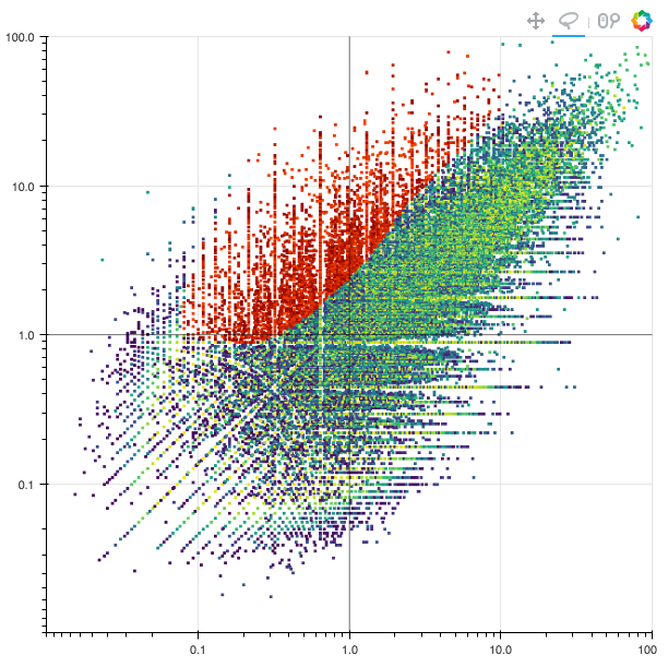
I had a need to plot more datapoints than Bokeh alone could handle. I started using datashader but needed the ability to lasso data. I was able to hack together a decent solution. I am including it below for anyone that may find it useful before InteractiveImage becomes part of Bokeh proper and thus integrated with the native lasso tool. The below code should work in jupyter with datashader 0.4.0 and Bokeh 0.12.4. I included a screen shot that shows the functionality post-lasso selection.
from datashader.bokeh_ext import InteractiveImage
from datashader.utils import export_image
from bokeh.models import Span, NumeralTickFormatter
from bokeh.models import LassoSelectTool, CustomJS
from bokeh.io import push_notebook
import pandas as pd
import numpy as np
plot_width=600
plot_height=600
x_range=(0.01,100)
y_range=(0.01,100)
scale = ‘log’
select_callback = CustomJS(code=’’’
console.log(cb_data.geometry)
var kernel = IPython.notebook.kernel;
var x = cb_data.geometry.x
var y = cb_data.geometry.y
var xs = JSON.stringify(Array.prototype.slice.call(x))
var ys = JSON.stringify(Array.prototype.slice.call(y))
kernel.execute(‘geometry_callback(’ + xs + ', '+ ys + ‘)’, {iopub: {output: function(o){console.log(o);}}}, {silent : false});
‘’’)
select = LassoSelectTool(select_every_mousemove=False, callback=select_callback)
p = figure(
plot_width=plot_width,

plot_height=plot_height,

x_range=x_range,

y_range=y_range,

x_axis_type=scale,

y_axis_type=scale,

tools=['pan', 'wheel_zoom', select],

toolbar_location='above')
Vertical line
vline = Span(location=1, dimension=‘height’, line_color=‘black’,
line_alpha=0.5, line_width=1)
Horizontal line
hline = Span(location=1, dimension=‘width’, line_color=‘black’,
line_alpha=0.5, line_width=1)
p.xaxis[0].formatter = NumeralTickFormatter(format=‘1,.0’)
p.yaxis[0].formatter = NumeralTickFormatter(format=‘1,.0’)
p.renderers.extend([vline, hline])
selected_df = df.head(0)
def geometry_callback(x, y):
#return x

global selected_df

global xc, xy, xycrop

xc = np.array(x)

yc = np.array(y)


xycrop = np.vstack((xc,yc)).T

path = Path(xycrop, closed=True)

selected_df = df.iloc[path.contains_points(df[['x', 'y']].values)]


p.yaxis[0].formatter = NumeralTickFormatter(format='1000.000')


InteractiveImage._callbacks[ii.ref].update({

    'xmin': _x_range[0],

    'xmax': _x_range[1],

    'ymin': _y_range[0],

    'ymax': _y_range[1],

    'w': _w,

    'h': _h

})

push_notebook()
(_x_range, _y_range, _w, _h) = (None, None, None, None)
def create_image(x_range, y_range, w=plot_width, h=plot_height):
global _x_range, _y_range, _w, _h


(_x_range, _y_range, _w, _h) = (x_range, y_range, w, h)

cvs = ds.Canvas(plot_width=plot_width, plot_height=plot_height, x_range=x_range, y_range=y_range, x_axis_type=scale, y_axis_type=scale)

agg = cvs.points(df, 'x', 'y', ds.sum('count'))

img = tf.shade(agg, cmap=viridis) #, how='eq_hist')


if selected_df.shape[0]:

    selected_agg = cvs.points(selected_df, 'x', 'y', ds.sum('count'))

    selected_shade = tf.shade(selected_agg, cmap=["darkred", 'orangered'])

    img = tf.stack(img, selected_shade)


return tf.dynspread(img, 0.5)# tf.spread(img, px=3) # tf.dynspread(img, 0.25)
selected_df = df.head(0)
ii=InteractiveImage(p, create_image)
ii