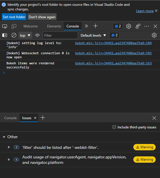
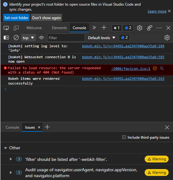
I’m practicing high dimensional dataset reduction techniques where the data is a file of 121 images. The problem I’m having is that when I run the command from the terminal, python -m bokeh serve --show, it returns a blank page. I think I messed up my callback functions or my plots but I can’t quite see the issue and how to solve it.
Heres what my code look likes.
import glob
import os
import numpy as np
from PIL import Image

from sklearn.manifold import TSNE
from umap import UMAP
from sklearn.decomposition import PCA

from bokeh.plotting import figure, curdoc
from bokeh.models import ColumnDataSource, Slider, ImageURL
from bokeh.layouts import layout, row, column
This is where I preprocess the data:
# Fetch the number of images using glob or some other path analyzer
N = len(glob.glob('static/*.jpg'))

# Find the root directory of your app to generate the image URL for the bokeh server
ROOT = os.path.split(os.path.abspath(os.path.dirname('__file__')))[1] + '/'

# Number of bins per color for the 3D color histograms
N_BINS_COLOR = 15

# Define an array containing the 3D color histograms. We have one histogram per image each having N_BINS_COLOR^3 bins.
# i.e. an N * N_BINS_COLOR^3 array
color_histograms = np.zeros((N,N_BINS_COLOR**3),dtype=int)

# initialize an empty list for the image file paths
url_list = []

# Compute the color and channel histograms
for idx, f in enumerate(glob.glob('static/*.jpg')):
    # open image using PILs Image package
    img = Image.open(f)

    # Convert the image into a numpy array and reshape it such that we have an array with the dimensions (N_Pixel, 3)
    a = np.asarray(img)
    a = a.reshape(a.shape[0]*a.shape[1], 3)

    # Compute a multi dimensional histogram for the pixels, which returns a cube
    H, edges = np.histogramdd(a,bins=N_BINS_COLOR)

    # However, later used methods do not accept multi dimensional arrays, so reshape it to only have columns and rows
    # (N_Images, N_BINS^3) and add it to the color_histograms array you defined earlier
    color_histograms[idx] = H.reshape(1, N_BINS_COLOR**3)

    # Append the image url to the list for the server
    url = ROOT + f
    url_list.append(url)

def compute_umap(n_neighbors=15) -> np.ndarray:
    """performes a UMAP dimensional reduction on color_histograms using given n_neighbors"""
    # compute and return the new UMAP dimensional reduction
    reduced_umap = UMAP(n_neighbors=n_neighbors).fit_transform(color_histograms)
    pass

    return reduced_umap

def on_update_umap(old, attr, new):
    """callback which computes the new UMAP mapping and updates the source_umap"""
    # Compute the new umap using compute_umap
    source_umap = compute_umap()

    # update the source_umap
    source_umap.data = source_umap

    pass

def compute_tsne(perplexity=4, early_exaggeration=10) -> np.ndarray:
    """performes a t-SNE dimensional reduction on color_histograms using given perplexity and early_exaggeration"""
    # compute and return the new t-SNE dimensional reduction
    reduced_tsne = TSNE(perplexity=perplexity,early_exaggeration=early_exaggeration).fit_transform(color_histograms)
    pass

    return reduced_tsne

def on_update_tsne(old, attr, new):
    """callback which computes the new t-SNE mapping and updates the source_tsne"""
    # Compute the new t-sne using compute_tsne
    source_tsne = compute_tsne()

    # update the source_tsne
    source_tsne.data = source_tsne

    pass
This is where I create my column data source:
# Calculate the indicated dimensionality reductions
pca_reduce = PCA(n_components=2).fit_transform(color_histograms)
tsne_reduce = compute_tsne()
umap_reduce = compute_umap()

# Construct three data sources, one for each dimensional reduction,
# each containing the respective dimensional reduction result and the image paths
source_pca = ColumnDataSource(dict(url=url_list,x=pca_reduce[:,0],y=pca_reduce[:,1]))
source_tsne = ColumnDataSource(dict(url=url_list,x=tsne_reduce[:,0],y=tsne_reduce[:,1]))
source_umap = ColumnDataSource(dict(url=url_list,x=umap_reduce[:,0],y=umap_reduce[:,1]))
This is where I create my plots
# Create a first figure for the PCA data. Add the wheel_zoom, pan and reset tools to it.
# And use bokehs image_url to plot the images as glyphs
pca_plot = figure(title='PCA',tools='wheel_zoom,pan,reset')
pca_plot.add_glyph(source_pca,ImageURL(url='url',x='x',y='y'))

# Create a second plot for the t-SNE result in the same fashion as the previous.
tsne_plot = figure(title='t-SNE',tools='wheel_zoom,pan,reset')
tsne_plot.add_glyph(source_tsne,ImageURL(url='url',x='x',y='y'))

# Create a third plot for the UMAP result in the same fashion as the previous.
umap_plot = figure(title='UMAP',tools='wheel_zoom,pan,reset')
umap_plot.add_glyph(source_umap,ImageURL(url='url',x='x',y='y'))
This is where I set my callbacks to update perplexity, early_exaggeration and n_neighbours
# Create a callback, such that whenever the value of the slider changes, on_update_tsne is called.
def tsne_callback(attr, old, new):

    perplexity = slider_perp.value_throttled
    source_tsne.data = on_update_tsne(perplexity=perplexity)

    pass

# Create a slider to control the t-SNE hyperparameter "perplexity" with a range from 2 to 20 and a title "Perplexity"
slider_perp = Slider(start=2, end=20, value=2, step=1, title='Perplexity')
slider_perp.on_change('value',tsne_callback)

# Create a second slider to control the t-SNE hyperparameter "early_exaggeration"
# with a range from 2 to 50 and a title "Early Exaggeration"
slider_early = Slider(start=2, end=50, value=2, step=1, title='Early Exaggeration')

# Connect it to the on_update_tsne callback in the same fashion as the previous slider
slider_early.on_change('value',on_update_tsne)

# Create a third slider to control the UMAP hyperparameter "n_neighbors"
slider_neigh = Slider(start=2, end=20, value=15, step=1, title='N Neighbors')

# Connect it to the on_update_umap callback in the same fashion as the previous slider
slider_neigh.on_change('value',on_update_umap)

lt = layout(column(row(pca_plot,tsne_plot,umap_plot),row(slider_perp,slider_early,slider_neigh)))
curdoc().add_root(lt)
curdoc().title = 'Title'
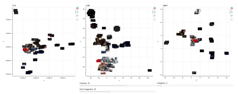
Expected output should look like so