Please note that the OLS and Theil-Sen results refer to the data points between the clicked x0 and x1. The Slope, Angle and Δy and Δx refer to the coordinates of the cliked points.
Bokeh Server:
import numpy as np
from bokeh.plotting import figure, curdoc
from bokeh.models import PointDrawTool, ColumnDataSource, HoverTool, Div, CustomAction, CustomJS
from scipy.stats import linregress, theilslopes
from bokeh.layouts import column
# ---- Generate random time series data ----
np.random.seed(0)
N = 30
x = np.arange(N)
y = np.cumsum(np.random.randn(N)) + 10 # random walk
# ---- Main plot ----
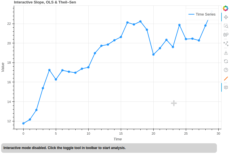
p = figure(width=800, height=500, title='Interactive Slope, OLS & Theil–Sen')
p.xaxis.axis_label = 'Time'
p.yaxis.axis_label = 'Value'
main_line = p.line(x, y, line_width=2, color="#08f", legend_label="Time Series")
p.circle(x, y, size=7, color="#08f", alpha=0.7)
# ---- Trend line for user selection ----
trend_source = ColumnDataSource(data={'x': [5, 20], 'y': [y[5], y[20]]})
trend_points = p.scatter(x='x', y='y', size=10, fill_color='orange', line_color='black', source=trend_source)
trend_line = p.line(x='x', y='y', line_color='orange', line_width=3, source=trend_source)
# Initially hide the interactive elements
trend_points.visible = False
trend_line.visible = False
draw_tool = PointDrawTool(renderers=[trend_points], add=False)
p.add_tools(draw_tool)
p.add_tools(HoverTool(tooltips=[('Time', '$x'), ('Value', '$y')], renderers=[main_line]))
results_div = Div(text="<b>Interactive mode disabled. Click the toggle tool in toolbar to start analysis.</b>",
width=1100, styles={'color': 'black', 'background-color': 'lightgray', 'padding':'8px', 'border-radius':'8px'})
# ---- Custom toolbar action with JavaScript callback ----
toggle_callback = CustomJS(
args=dict(
trend_points=trend_points,
trend_line=trend_line,
draw_tool=draw_tool,
results_div=results_div,
plot=p
),
code="""
// Toggle visibility
const currently_visible = trend_points.visible;
trend_points.visible = !currently_visible;
trend_line.visible = !currently_visible;
// Toggle active tool
if (!currently_visible) {
// Enable interactive mode
plot.toolbar.active_tap = draw_tool;
results_div.text = "<b>Interactive mode enabled! Drag the red endpoints to analyze different segments.</b>";
} else {
// Disable interactive mode
plot.toolbar.active_tap = null;
results_div.text = "<b>Interactive mode disabled. Click the toggle tool in toolbar to start analysis.</b>";
}
"""
)
# Create custom action for toolbar
toggle_action = CustomAction(
icon="data:image/svg+xml;base64,PHN2ZyB3aWR0aD0iMjQiIGhlaWdodD0iMjQiIHZpZXdCb3g9IjAgMCAyNCAyNCIgZmlsbD0ibm9uZSIgeG1sbnM9Imh0dHA6Ly93d3cudzMub3JnLzIwMDAvc3ZnIj4KICA8cGF0aCBkPSJNNCAyMEwyMCA0IiBzdHJva2U9IiNmZjY2MDAiIHN0cm9rZS13aWR0aD0iMyIgc3Ryb2tlLWxpbmVjYXA9InJvdW5kIi8+Cjwvc3ZnPgo=",
description="Toggle Interactive Mode",
callback=toggle_callback
)
p.add_tools(toggle_action)
# ---- Div for slope display ----
results_div = Div(text="<b>Interactive mode disabled. Click the toggle tool in toolbar to start analysis.</b>",
width=750, styles={'color': 'black', 'background-color': 'lightgray', 'padding':'8px', 'border-radius':'8px'})
def update_div(attr, old, new):
# Note: This will work when interactive mode is enabled via JavaScript
xs = trend_source.data['x']
ys = trend_source.data['y']
if len(xs) != 2 or len(ys) != 2:
results_div.text = "<b>Drag endpoints. Slope, OLS, Theil–Sen will show here.</b>"
return
x0, x1 = xs[0], xs[1]
y0, y1 = ys[0], ys[1]
idx0, idx1 = int(round(x0)), int(round(x1))
if idx0 == idx1 or not (0 <= idx0 < N and 0 <= idx1 < N):
results_div.text = "<b>Select two <i>different</i> points within range.</b>"
return
lo, hi = sorted([idx0, idx1])
x_sel = x[lo:hi+1]
y_sel = y[lo:hi+1]
if len(x_sel) > 1:
ols = linregress(x_sel, y_sel).slope
ols_pv = linregress(x_sel, y_sel).pvalue
theil = theilslopes(y_sel, x_sel)[0]
else:
ols = np.nan
theil = np.nan
dx = x1 - x0
dy = y1 - y0
if dx != 0:
slope = dy / dx
slope_str = f"Slope = {slope:.3f}"
else:
slope_str = "Slope = ∞"
angle = (180/np.pi) * np.arctan2(dy, dx)
results_div.text = (
f"<b>x0 = {x0:.2f}, y0 = {y0:.2f}, x1 = {x1:.2f}, y1 = {y1:.2f}, Δx = {dx:.2f}, Δy = {dy:.2f}, {slope_str}, Angle = {angle:.2f}°<br>"
f"OLS Slope = {ols:.3f}, OLS p-value = {ols_pv:.5f}, Theil–Sen Slope = {theil:.3f}</b>"
)
trend_source.on_change('data', update_div)
curdoc().add_root(column(p, results_div))
curdoc().title = "Interactive Timeseries Slope"
Without Server:
import numpy as np
from bokeh.plotting import figure, show, output_file
from bokeh.models import PointDrawTool, ColumnDataSource, HoverTool, Div, CustomAction, CustomJS
from bokeh.layouts import column

# Generate random time series data
np.random.seed(0)
N = 30
x = np.arange(N)
y = np.cumsum(np.random.randn(N)) + 10  # random walk

p = figure(width=800, height=500, title='Interactive Δx, Δy, Slope')
p.xaxis.axis_label = 'Time'
p.yaxis.axis_label = 'Value'
main_line = p.line(x, y, line_width=2, color="#08f")
p.circle(x, y, size=7, color="#08f", alpha=0.7)

trend_source = ColumnDataSource(data={'x': [5, 20], 'y': [y[5], y[20]]})
trend_points = p.scatter(x='x', y='y', size=10, fill_color='orange', line_color='black', source=trend_source)
trend_line = p.line(x='x', y='y', line_color='orange', line_width=3, source=trend_source)

trend_points.visible = False
trend_line.visible = False

draw_tool = PointDrawTool(renderers=[trend_points], add=False)
p.add_tools(draw_tool)
p.add_tools(HoverTool(tooltips=[('Time', '$x'), ('Value', '$y')], renderers=[main_line]))

results_div = Div(
    text="<b>Interactive mode disabled. Click the toggle tool in toolbar to start analysis.</b>",
    width=800, styles={'color': 'black', 'background-color': 'lightgray', 'padding': '8px', 'border-radius': '8px'}
)

# --- JS callback for updating results_div with dx, dy, slope ---
update_callback = CustomJS(
    args=dict(
        trend_source=trend_source,
        results_div=results_div
    ),
    code="""
    const xs = trend_source.data.x, ys = trend_source.data.y;
    if (xs.length != 2 || ys.length != 2) {
        results_div.text = "<b>Drag endpoints. Slope will show here.</b>";
        return;
    }
    let x0 = xs[0], x1 = xs[1], y0 = ys[0], y1 = ys[1];
    let dx = x1 - x0, dy = y1 - y0;
    let slope_str;
    if (dx != 0) {
        let slope = dy / dx;
        slope_str = "Slope = " + slope.toFixed(3);
    } else {
        slope_str = "Slope = ∞";
    }
    results_div.text = `<b>Δx = ${dx.toFixed(2)}, Δy = ${dy.toFixed(2)}, ${slope_str}</b>`;
    """
)
trend_source.js_on_change('data', update_callback)

# --- Toolbar toggle button for interactive mode ---
toggle_callback = CustomJS(
    args=dict(
        trend_points=trend_points,
        trend_line=trend_line,
        draw_tool=draw_tool,
        results_div=results_div,
        plot=p
    ),
    code="""
    const currently_visible = trend_points.visible;
    trend_points.visible = !currently_visible;
    trend_line.visible = !currently_visible;
    if (!currently_visible) {
        plot.toolbar.active_tap = draw_tool;
        results_div.text = "<b>Interactive mode enabled! Drag the orange endpoints to analyze.</b>";
    } else {
        plot.toolbar.active_tap = null;
        results_div.text = "<b>Interactive mode disabled. Click the toggle tool in toolbar to start analysis.</b>";
    }
    """
)
toggle_action = CustomAction(
    icon="data:image/svg+xml;base64,PHN2ZyB3aWR0aD0iMjQiIGhlaWdodD0iMjQiIHZpZXdCb3g9IjAgMCAyNCAyNCIgZmlsbD0ibm9uZSIgeG1sbnM9Imh0dHA6Ly93d3cudzMub3JnLzIwMDAvc3ZnIj4KICA8cGF0aCBkPSJNNCAyMEwyMCA0IiBzdHJva2U9IiNmZjY2MDAiIHN0cm9rZS13aWR0aD0iMyIgc3Ryb2tlLWxpbmVjYXA9InJvdW5kIi8+Cjwvc3ZnPgo=",
    description="Toggle Interactive Mode",
    callback=toggle_callback
)
p.add_tools(toggle_action)

output_file("minimal_slope_interactive.html")
show(column(p, results_div))