Lasso/Box select tool plot interaction between scatter plot and histogram

Hello everyone. I’m working on an exercise where a lasso and/or box select tool highlights the area of a histogram according to what was selected on a scatter plot. The problem I’m facing is that the histogram won’t fill the colors for the respective selection. I believe I’m not implementing the interactions correctly. Here is my full code below.

Import required libraries

import pandas as pd
import numpy as np
from bokeh.io import output_file, show, save,curdoc, output_notebook
from bokeh.plotting import figure
from bokeh.models import ColumnDataSource, HoverTool,FactorRange, NumeralTickFormatter,HBar, DatetimeTickFormatter
from bokeh.models.widgets import Select
from bokeh.layouts import column, row, gridplot
import bokeh.palettes as bp # uncomment it if you need special colors that are pre-defined
import datetime as dt
from math import pi
from bokeh.layouts import gridplot
from bokeh.models import BoxSelectTool, LassoSelectTool

Some dummy data

print(df_scatterplot.head(50))
         dates  trip_duration  passenger_count vendor_id    color
0   2016-01-01            257                1  vendor_2  #32CD32
1   2016-01-01             86                2  vendor_2  #32CD32
2   2016-01-01           1147                1  vendor_2  #32CD32
3   2016-01-01            540                1  vendor_1  #FF0000
4   2016-01-01            411                1  vendor_1  #FF0000
5   2016-01-01            227                2  vendor_2  #32CD32
6   2016-01-01            474                1  vendor_2  #32CD32
7   2016-01-01            473                1  vendor_1  #FF0000
8   2016-01-01            654                1  vendor_2  #32CD32
9   2016-01-01            295                1  vendor_1  #FF0000
10  2016-01-01             69                1  vendor_1  #FF0000
11  2016-01-01            286                2  vendor_2  #32CD32
12  2016-01-01            998                1  vendor_2  #32CD32
13  2016-01-01            928                1  vendor_1  #FF0000
14  2016-01-01            295                2  vendor_2  #32CD32
15  2016-01-01            338                1  vendor_2  #32CD32
16  2016-01-02           1195                2  vendor_1  #FF0000
17  2016-01-02            407                2  vendor_2  #32CD32
18  2016-01-02           1898                1  vendor_1  #FF0000
19  2016-01-02            945                1  vendor_1  #FF0000
20  2016-01-02            223                2  vendor_2  #32CD32
21  2016-01-02           1141                1  vendor_1  #FF0000
22  2016-01-02            219                2  vendor_2  #32CD32
23  2016-01-02            290                1  vendor_2  #32CD32
24  2016-01-02            376                3  vendor_2  #32CD32
25  2016-01-02            632                1  vendor_1  #FF0000
26  2016-01-02            254                1  vendor_1  #FF0000
27  2016-01-03           1379                1  vendor_2  #32CD32
28  2016-01-03            745                1  vendor_1  #FF0000
29  2016-01-03            349                2  vendor_2  #32CD32
30  2016-01-03            540                3  vendor_2  #32CD32
31  2016-01-03            243                1  vendor_1  #FF0000
32  2016-01-03            731                1  vendor_1  #FF0000
33  2016-01-03           1388                1  vendor_1  #FF0000
34  2016-01-03            720                1  vendor_1  #FF0000
35  2016-01-03           1197                1  vendor_1  #FF0000
36  2016-01-03            512                1  vendor_2  #32CD32
37  2016-01-03            510                1  vendor_1  #FF0000
38  2016-01-03            751                6  vendor_2  #32CD32
39  2016-01-03            112                1  vendor_2  #32CD32
40  2016-01-03            424                6  vendor_2  #32CD32
41  2016-01-03            228                1  vendor_1  #FF0000
42  2016-01-03            819                1  vendor_1  #FF0000
43  2016-01-03            862                1  vendor_2  #32CD32
44  2016-01-03            828                1  vendor_1  #FF0000
45  2016-01-04           1238                1  vendor_2  #32CD32
46  2016-01-04            872                1  vendor_1  #FF0000
47  2016-01-04           1101                4  vendor_1  #FF0000
48  2016-01-04            649                6  vendor_2  #32CD32
49  2016-01-04            743                1  vendor_1  #FF0000

Here I create my ColumnDataSource, scatterplot, hover tools and selection tools.

data = {'Dates': list(df_scatterplot['dates']),
        'TripDuration': list(df_scatterplot['trip_duration']),
        'NumOfPass': list(df_scatterplot['passenger_count']),
        'Vendor': list(df_scatterplot['vendor_id']),
        'Color' : list(df_scatterplot['color'])
       }
source_scatter = ColumnDataSource(data)

x_Range = list(dict.fromkeys(source_scatter.data['Dates']))

TOOLS="lasso_select, box_select, reset"

p = figure(tools=TOOLS, plot_width=3000, plot_height=900,
           toolbar_location="above",x_range = x_Range,
           title="NYC Taxi Traffic")

p.yaxis.axis_label = "Trip Duration (seconds)"
p.xaxis.axis_label = "Dates"
p.xaxis.major_label_orientation = pi/4
p.xaxis.major_label_text_font_size = '8px'
p.xgrid.grid_line_color = None
p.ygrid.grid_line_color = None
p.sizing_mode = "stretch_both"
p.select(LassoSelectTool).select_every_mousemove = False
p.select(BoxSelectTool).select_every_mousemove = False

hover = HoverTool(tooltips = [
    ('Date','@Dates'),
    ('Trip Duration','@TripDuration'),
    ('Number of Passengers','@NumOfPass'),
    ('Vendor ID','@Vendor')
])
p.add_tools(hover)

scatter = p.scatter(x='Dates',y='TripDuration',size='NumOfPass',color='Color',source=source_scatter)

Here I create my histogram for the trip duration. This is also where I have some bokeh warnings.

hhist, hedges = np.histogram(a=df_scatterplot['trip_duration'],bins=20)

hzeros = np.zeros(len(hedges)-1)
hmax = max(hhist)*1.1

LINE_ARGS1 = dict(color="#ffbdbd", line_color=None)
LINE_ARGS2 = dict(color="#d9f5d9", line_color=None)

ph = figure(title="Histogram", tools='', background_fill_color="#fafafa", plot_width=1500, plot_height=200, x_range=p.y_range, y_range=(0, hmax))
ph.xgrid.grid_line_color = None
ph.yaxis.major_label_orientation = np.pi/4

ph.quad(top=hhist,bottom=hzeros,left=hedges[:-1],right=hedges[1:],fill_color='white', line_color='navy')
ph.y_range.start = 0
ph.yaxis.axis_label = "Number of Trips"
ph.xaxis.axis_label = "Trip Duration"

# Create two more histogram quads for selected data. 
# These two quads will be manipulated by the selection tools. When we select data from the scatter plot, we want histogram to be highlighted with the parts that
# corresponds to our data points. Therefore, we need two more quads to indicate the highlighted area. The color will be the same but we will 
# use the alpha value = 0.5 

hh1 = ph.quad(top=source_scatter.selected.indices,bottom=hzeros,left=hedges[:-1],right=hedges[1:], alpha=0.5,**LINE_ARGS1)
hh2 = ph.quad(top=source_scatter.selected.indices,bottom=hzeros,left=hedges[:-1],right=hedges[1:], alpha=0.5,**LINE_ARGS2)
BokehUserWarning: ColumnDataSource's columns must be of the same length. Current lengths: ('bottom', 20), ('top', 0)
BokehUserWarning: ColumnDataSource's columns must be of the same length. Current lengths: ('bottom', 20), ('left', 20), ('top', 0)
BokehUserWarning: ColumnDataSource's columns must be of the same length. Current lengths: ('bottom', 20), ('left', 20), ('right', 20), ('top', 0)

Finally the update function and layout creation.

# Implement the update function that will be triggered when the lasso or box selection tool is used.
def update(attr, old, new):
    nds = new  # index of the data that are selected
    hh1.selected.nds
    hh2.selected.nds
    pass

scatter.data_source.selected.on_change('indices', update)

layout = column(p, row(ph))
curdoc().add_root(layout)

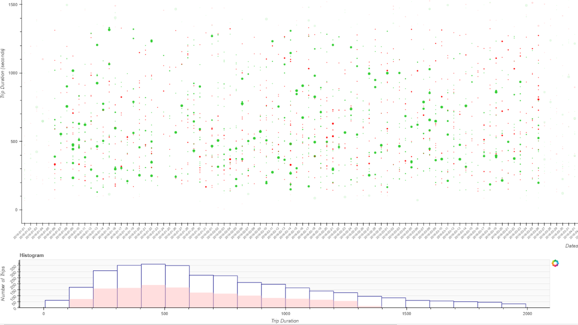
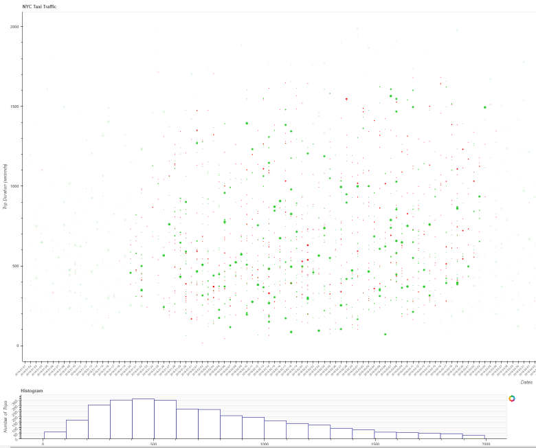
The following plot produces after using the lasso tool

cd path
bokeh serve --show code_file.ipynb

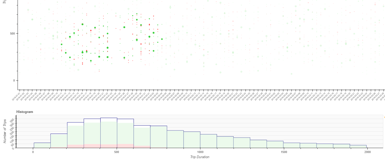
However, the histogram should be filled after my select with one of the tools like so


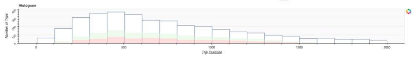
Where did I go wrong in my code above? I’m sure it’s very minor but I can’t see it. Thanks in advance.

Happy to be corrected, but I think you’re missing more to your code than you think.

On selection, you currently aren’t binning the selected data. How does your script know what height to make each bin when the user makes an arbitrary selection of points? You’ll need to re-tally how many data points live in each bin. Then with that done, you need to further split each bin up to tally within the count of each vendor. THEN, you need to recalculate the geometry of the quads based on some sort of cumulative summing to “stack” the different colors.

But even all that aside,

hh1 = ph.quad(top=source_scatter.selected.indices,bottom=hzeros,left=hedges[:-1],right=hedges[1:], alpha=0.5,**LINE_ARGS1)
hh2 = ph.quad(top=source_scatter.selected.indices,bottom=hzeros,left=hedges[:-1],right=hedges[1:], alpha=0.5,**LINE_ARGS2)

Doesn’t make sense. You’re getting the bokeh warnings because on initialization source_scatter.selected.indices is an empty array, and if you make a selection of say 7 points, source.selected.indices will return an array of the indices of the those points (i.e. it will be 7 long), when what you actually want is an array that’s always as long as the number of bins (20 in your case if you only had one vendor, but multiply 20 by the number of vendors you have because each quad needs one record in the CDS). On init you’ll want to pass an array of 0s of that length because it starts with nothing selected, but when you implement the whole retallying and stacking logic I outlined above, you’ll update those values with new geometry.

My advice would be to start small, and figure out the tallying by duration part first (don’t think about vendor “stacking” at all). Then with that in hand start working on splitting it up further. Since you’re using python-side callbacks, pandas’ groupby and cut methods are gonna be your best friend for this :slight_smile: Good luck!

1 Like

Ok thanks for your input. I was able to get it to work. However, the quads are only one color. I’m missing something in the callback I believe. So,
I changed this

hh1 = ph.quad(top=source_scatter.selected.indices,bottom=hzeros,left=hedges[:-1],right=hedges[1:], alpha=0.5,**LINE_ARGS1)
hh2 = ph.quad(top=source_scatter.selected.indices,bottom=hzeros,left=hedges[:-1],right=hedges[1:], alpha=0.5,**LINE_ARGS2)

to this

hh1 = ph.quad(top=hzeros,bottom=0,left=hedges[:-1],right=hedges[1:],alpha=0.5,**LINE_ARGS1)
hh2 = ph.quad(top=hzeros,bottom=0,left=hedges[:-1],right=hedges[1:],alpha=0.5,**LINE_ARGS2)

And I updated my callback function from this

def update(attr, old, new):
    nds = new  # index of the data that are selected
    hh1.selected.nds
    hh2.selected.nds
    pass

to this

def update(attr, old, new):
    nds = new  # index of the data that are selected
    if len(nds) == 0 or len(nds) == len(df_scatterplot['trip_duration']):
        hhist1, hhist2 = hzeros, hzeros
    else:
        neg_nds = np.ones_like(df_scatterplot['trip_duration'], dtype=np.bool)
        neg_nds[nds] = False
        hhist1, _ = np.histogram(df_scatterplot['trip_duration'][nds], bins=hedges)
        hhist2, _ = np.histogram(df_scatterplot['trip_duration'][neg_nds], bins=hedges)

    hh1.data_source.data['top'] = hhist1
    hh2.data_source.data['top'] = -hhist2
    pass

So the lasso and box tool is working but I’m just missing something with the color.


@gmerritt123
bokeh/selection_histogram.py at branch-3.0 · bokeh/bokeh · GitHub

Getting closer! Looks to me like you’ve got the the duration binning figured out, but what remains is to further split each bin into counts for each vendor type, and then calculating new geometries based on “stacking” the vendors in each bin.

I’m definitely closer now, but for some reason, the whole histograms fill with green even with the smallest amount selected.

hh1 = ph.quad(top=hzeros,bottom=hzeros,left=hedges[:-1],right=hedges[1:],alpha=0.5,**LINE_ARGS1)
hh2 = ph.quad(top=hzeros,bottom=hzeros,left=hedges[:-1],right=hedges[1:],alpha=0.5,**LINE_ARGS2)
def update(attr, old, new):
    nds = new  # index of the data that are selected
    if len(nds) == 0 or len(nds) == len(df_scatterplot['trip_duration']):
        hhist1, hhist2 = hzeros, hzeros
    else:
        neg_nds = np.ones_like(df_scatterplot['trip_duration'], dtype=np.bool)
        neg_nds[nds] = False
        hhist1, hedges1 = np.histogram(df_scatterplot['trip_duration'][nds], bins=hedges)
        hhist2, hedges2 = np.histogram(df_scatterplot['trip_duration'][neg_nds], bins=hedges)
        
    hzeros1 = np.zeros(len(hedges1)-1)
    hzeros2 = np.zeros(len(hedges2)-1)

    hh1.data_source.data['top'] = hhist1
    hh2.data_source.data['top'] = hhist2
    
    hh1.data_source.data['bottom'] = hzeros1
    hh2.data_source.data['bottom'] = hhist1
    pass


@gmerritt123

I think you’re trying too hard to copy/follow an example from the docs without thinking about how the example differs from what you’re actually trying to do. The example you’re referring to is not doing the stacking you need to do, yet your code makes no attempt.

See this example below that essentially does the aggregation and stacking for you. Please read up on pd.cut and pd.groupby as I’ve suggested → it is absolutely key to this setup. Of course you could fundamentally stick to np.histogram but why would you since you also need to group by a categorical in order to perform the stacking operation.

import pandas as pd
import numpy as np
from bokeh.plotting import figure, show
from bokeh.models import ColumnDataSource

#make a normal dist w random noise
dl = np.random.normal(50,10,1000)+np.random.random(1000)*2
#assign a categorical
fruits = ['banana' for x in range(400)]+['apple' for x in range(300)]+['orange' for x in range(300)]
#make a dataframe of this
df = pd.DataFrame(data={'duration':dl,'fruit':fruits})


def agg_and_stack(df):
    '''assembles a datasource for quad'''
    colormapping = {'apple':'red','banana':'yellow','orange':'orange'} #for making a colorfield --> there are slicker ways to do this but this straightforward
    #READ ABOUT pd.groupby and pd.cut! This groups the dataframe into 10 evenly spaced bins by duration, AND by fruit... AND aggregates by counting the number of records in each group
    gb = df.groupby([pd.cut(df['duration'],10),'fruit']).count().rename(columns={'duration':'count'}).reset_index()
    #get the left and right bounds of each duration bin
    gb['left'] = [x.left for x in gb['duration']]
    gb['right'] = [x.right for x in gb['duration']]
    #getting the top, need to take a cumulative sum within each duration bin, and then 
    gb['top'] = gb.groupby('left')['count'].cumsum()
    #to get the bottom, need to basically take the previous top, and assign 0 to the bottommost bottom
    gb['bottom'] = gb.groupby('left')['top'].shift(1).fillna(0)
    #map the colors
    gb['clr'] = gb['fruit'].map(colormapping)
    #assemble a dictionary to update cds data
    data = {x:np.array(gb[x]) for x in ['fruit','left','right','top','bottom','clr']}
    return data

cds = ColumnDataSource(data=agg_and_stack(df))

f=figure()
r = f.quad(top='top',bottom='bottom',left='left',right='right',fill_color='clr',source=cds,legend_field='fruit')
show(f)

Now to implement this in your callback, you’d take the selected indices, filter the df down to only those indices, then perform my little routine, then update the quad’s datasource with “data” (i.e. the dictionary that my function is currently returning).

Solved it. I just had to change my update function to the following.

def update(attr, old, new):
    nds = new
    if len(nds) == 0 or len(nds) == len(df_scatterplot['trip_duration']):
        hhist1, hhist2 = hzeros, hzeros
    else:
        hhist1, hedges1 = np.histogram(df_scatterplot['trip_duration'][nds][df_scatterplot['vendor_id']=='vendor_1'], bins=hedges)
        hhist2, hedges2 = np.histogram(df_scatterplot['trip_duration'][nds][df_scatterplot['vendor_id']=='vendor_2'], bins=hedges)
        
    hzeros1 = np.zeros(len(hedges1)-1)
    hzeros2 = np.zeros(len(hedges2)-1)

    hh1.data_source.data['top'] = hhist1
    hh2.data_source.data['top'] = hhist2 + hhist1
    
    hh1.data_source.data['bottom'] = hzeros1
    hh2.data_source.data['bottom'] = hhist1
    pass
1 Like

This topic was automatically closed 90 days after the last reply. New replies are no longer allowed.