Nested axis for heatmap chart

I am trying to create a heatmap chart with nested axis, similar to this one but for heatmaps instead of bar charts.
Here is the code I came up with, but I don’t seem to be able to pass tuples as factors?

from bokeh.layouts import row
from bokeh.plotting import figure, show, output_file
from itertools import product

factors_x = ["A", "B", "C"]
factors_y = [["Category1","1"], ["Category1","2"], ["Category1","3"],["Category2","X"], ["Category2","Y"], ["Category3","?"]]
#it works well if I uncomment the following line
#factors_y=[a[1] for a in factors_y]

x=[a[0] for a in product(factors_x,factors_y)]
y=[a[1] for a in product(factors_x,factors_y)]
values=np.random.uniform(size=(len(x),))
colors=['#%02x%02x%02x' % (255,255-int(255*i),0) for i in values]

hm = figure(title="Categorical Heatmap", tools="hover", toolbar_location=None,
            x_range=factors_x, y_range=factors_y)

hm.rect(x, y, color=colors, width=1, height=1)

show(hm)

Many thanks

Hi ahassaine,

I was able to get your code working by pre-declaring the FactorRange for the y_range with the tuples list.

from bokeh.plotting import figure, show
from bokeh.models import FactorRange
from itertools import product
import numpy as np

factors_x = ["A", "B", "C"]
factors_y = [("Category1", "1"), ("Category1", "2"), ("Category1", "3"),
             ("Category2", "X"), ("Category2", "Y"), ("Category3", "?")]

x = [a[0] for a in product(factors_x, factors_y)]
y = [a[1] for a in product(factors_x, factors_y)]

values = np.random.uniform(size=(len(x),))
colors = ['#%02x%02x%02x' % (255, 255-int(255*i), 0) for i in values]

y_range = FactorRange(factors=factors_y)
hm = figure(title="Categorical Heatmap", tools="hover", toolbar_location=None,
            x_range=factors_x, y_range=y_range)
hm.rect(x, y, color=colors, width=1, height=1)
hm.y_range.group_padding = 0

show(hm)

Note that you’ll also want to set the group_padding to 0, otherwise you’ll have gaps between the cells.

2 Likes

Many thanks for this!

I am working in the same field: categorical heatmaps with callbacks. I am not able to change the number of elements in the categorical axis according to changes in widgets. It seems that after you define y-range initially, that values are not updating as changes in widgets. My question is how to change the y_range values interactively. Thank you very much for your kind help. My code is:

   ##FUNCTIONS:
    def get_dataset(src, product_selec, wash_selec, process_selec, monitor_selec):
        dfff = src[src["PRODUCT"].isin(product_selec) & src["WASH"].isin(wash_selec) & src["PROCESS"].isin(process_selec) & src["MONITOR"].isin(monitor_selec)]
        dfff = dfff.groupby(['MODALITY', 'SCENARIOS', 'WASH', 'PROCESS', 'PRODUCT', 'MONITOR', 'INDEX', 'DIVERSE_SCENARIOS'])[['SRI']].mean().round(2)
        dfff.reset_index(inplace=True)
        source = ColumnDataSource(dfff)
        source.remove('index')
        return source
    ##
    ##
    ##SET UP CALLBACKS
    def update_plot(attr, old, new):
        src = get_dataset(dff_stacked, mc_product.value, mc_wash.value, mc_process.value, mc_monitor.value)
        ch.data_source.data=dict(src.data)
    ##
    ##

Original data: dataframe named dff_stacked

    l_products = list(dff_stacked.PRODUCT.unique())
    l_washes = list(dff_stacked.WASH.unique())
    l_processes = list(dff_stacked.PROCESS.unique())
    l_monitors = list(dff_stacked.MONITOR.unique())
    ##
    source = get_dataset(dff_stacked, list(l_products), list(l_washes[:1]), list(l_processes[:1]), list(l_monitors[:2]))
    ##
    plot = figure(x_range=np.unique(source.data['DIVERSE_SCENARIOS']), y_range=np.unique(source.data['PRODUCT']), x_axis_location="above", toolbar_location=None, tools="", plot_width=1200, plot_height=600)
    # plot = figure(x_range=dff_stacked.DIVERSE_SCENARIOS.unique(), y_range=dff_stacked.PRODUCT.unique(), x_axis_location="above", toolbar_location=None, tools="", plot_width=1200, plot_height=600)        
    ##
    mapper = LinearColorMapper(palette=list(reversed(cc.b_rainbow_bgyr_35_85_c72)), low=80, high=100) 
    ##      
    ch = plot.rect(x="DIVERSE_SCENARIOS", y="PRODUCT", width=1, height=1, source=source, line_color=None, fill_color=transform('SRI', mapper))           
    color_bar = ColorBar(color_mapper=mapper, location=(0, 0), ticker=BasicTicker(desired_num_ticks=10), title='SRI')
    ##
    plot.add_layout(color_bar, 'right')

… some additional code, then:

    # ## SET UP WIDGETS AND CALLBACKS
    mc_product = MultiChoice(value=list(l_products[:3]), options=l_products)
    mc_wash = MultiChoice(value=list(l_washes[:1]), options=l_washes)
    mc_process = MultiChoice(value=list(l_processes[:1]), options=l_processes)
    mc_monitor = MultiChoice(value=list(l_monitors[:2]), options=l_monitors)
    # ##
    # ##        
    for w in [mc_product, mc_wash, mc_process, mc_monitor]:
        w.on_change('value', update_plot)
    # ##
    # ##

Hi @CONSUMERTEC,

I’m happy to take a look, but could you reformat your code sample as a minimal, reproducible example? The idea is that someone (like me) could copy and paste it all at once, including all necessary imports and data sources, and then see what you see.

Hello Carolyn,
Thank you for your kind response. Below you will find the full code and I am uploading the original table to graph. As you will see it is Flask code that include Bokeh code, and you can run from Visual Code. Thank you for your time on this.

import pandas as pd
import numpy as np
import colorcet as cc
from threading import Thread

from flask import Flask, render_template
from tornado.ioloop import IOLoop

from bokeh.plotting import figure
from bokeh.layouts import column, row
from bokeh.models import HoverTool, BasicTicker, ColorBar, ColumnDataSource, LinearColorMapper, PrintfTickFormatter, MultiChoice, CustomJS
from bokeh.themes import Theme
from bokeh.embed import components
from bokeh.resources import CDN
from bokeh.transform import linear_cmap, factor_cmap, transform
from bokeh.palettes import palettes, mpl
from bokeh.embed import server_document, server_session
from bokeh.server.server import Server
from bokeh.client import pull_session

app = Flask(name)

@app.route(’/’, methods=[‘GET’])
def bkapp_page():

def bkapp(doc):

    data_url = '(PATH TO BE CHANGED).csv'
    df_ini = pd.read_csv(data_url)
    ##
    df = df_ini.copy()
    ##
    ## PREPARACION DE LA TABLA
    ## RETIRO DEL LAVADO 00_00
    dff = df[~(df['WASH'].isin(['00_00']))]
    ## STACK DE LOS INDICES
    dff_stacked = pd.melt(dff, id_vars=['MODALITY', 'SCENARIOS', 'WASH', 'PROCESS', 'PRODUCT', 'MONITOR'], value_vars=['1.2.SRI_STw', '2.2.SRI_LIw', '3.2.SRI_HUw', '4.2.SRI_CRw'], var_name='INDEX', value_name='SRI')
    ## CREACION DE COLUMNA DE TODOS LOS ESCENARIOS
    dff_stacked['DIVERSE_SCENARIOS'] = dff_stacked['MODALITY'] + dff_stacked['SCENARIOS'] + dff_stacked['INDEX']
    ## AGRUPACION Y MEDIA DE LAS REPLICAS
    dff_stacked = dff_stacked.groupby(['MODALITY', 'SCENARIOS', 'WASH', 'PROCESS', 'PRODUCT', 'MONITOR', 'INDEX', 'DIVERSE_SCENARIOS'])[['SRI']].mean().round(2)
    dff_stacked.reset_index(inplace=True)
    ##
    ##
    ##SET DATA
    def get_dataset(src, product_selec, wash_selec, process_selec, monitor_selec):
        dfff = src[src["PRODUCT"].isin(product_selec) & src["WASH"].isin(wash_selec) & src["PROCESS"].isin(process_selec) & src["MONITOR"].isin(monitor_selec)]
        dfff = dfff.groupby(['MODALITY', 'SCENARIOS', 'WASH', 'PROCESS', 'PRODUCT', 'MONITOR', 'INDEX', 'DIVERSE_SCENARIOS'])[['SRI']].mean().round(2)
        dfff.reset_index(inplace=True)
        source = ColumnDataSource(dfff)
        source.remove('index')
        print(len(src), len(dfff), 'datos')
        return source
    ##
    ##
    ##SET UP CALLBACKS
    def update_plot(attr, old, new):
        src = get_dataset(dff_stacked, mc_product.value, mc_wash.value, mc_process.value, mc_monitor.value)
        # source.data.update(src.data)
        ch.data_source.data=dict(src.data)
        plot.y_range = np.unique(src.data['PRODUCT'])
    ##
    ##
    ########################
    ######################## 
    ## INICIO DEL GRAFICO
    l_products = list(dff_stacked.PRODUCT.unique())
    l_washes = list(dff_stacked.WASH.unique())
    l_processes = list(dff_stacked.PROCESS.unique())
    l_monitors = list(dff_stacked.MONITOR.unique())
    ##
    source = get_dataset(dff_stacked, list(l_products), list(l_washes[:1]), list(l_processes[:1]), list(l_monitors[:2]))
    ##
    plot = figure(x_range=np.unique(source.data['DIVERSE_SCENARIOS']), y_range=np.unique(source.data['PRODUCT']), x_axis_location="above", toolbar_location=None, tools="", plot_width=1200, plot_height=600)
    # plot = figure(x_range=dff_stacked.DIVERSE_SCENARIOS.unique(), y_range=dff_stacked.PRODUCT.unique(), x_axis_location="above", toolbar_location=None, tools="", plot_width=1200, plot_height=600)        
    ##
    mapper = LinearColorMapper(palette=list(reversed(cc.b_rainbow_bgyr_35_85_c72)), low=80, high=100) 
    ##      
    ch = plot.rect(x="DIVERSE_SCENARIOS", y="PRODUCT", width=1, height=1, source=source, line_color=None, fill_color=transform('SRI', mapper))           
    color_bar = ColorBar(color_mapper=mapper, location=(0, 0), ticker=BasicTicker(desired_num_ticks=10), title='SRI')
    ##
    plot.add_layout(color_bar, 'right')
    ##
    plot.title.text = "Graph: Stain Removal Index (SRI) by Product. Each value is presented by a coloured tile/retangle according to a colorscale. Values >94-95 = Total cleanliness. Values between 90-94 = Conditional cleanliness, see virtual reality on consumer garments. Diverse Scenarios combines: adopted whites, illuminants, surrounds, observers and visual sensitivity"
    plot.title.align = "left"
    plot.title.text_color = "black"
    plot.title.text_font_size = "14px"
    plot.axis.axis_line_color = None
    plot.axis.major_tick_line_color = None
    plot.axis.major_label_text_font_size = "12px"
    plot.axis.major_label_standoff = 0
    plot.xaxis.major_label_orientation = 1.0
    ##
    ##
    # ## SET UP WIDGETS AND CALLBACKS
    mc_product = MultiChoice(value=list(l_products[:3]), options=l_products)
    mc_wash = MultiChoice(value=list(l_washes[:1]), options=l_washes)
    mc_process = MultiChoice(value=list(l_processes[:1]), options=l_processes)
    mc_monitor = MultiChoice(value=list(l_monitors[:2]), options=l_monitors)
    # ##
    # ##        
    for w in [mc_product, mc_wash, mc_process, mc_monitor]:
        w.on_change('value', update_plot)
    # ##
    # ##
    ########################
    ########################        
    ## SET UP LAYOUT AND ADD TO DOCUMENT
    inputs = row(mc_product, mc_wash, mc_process, mc_monitor)
    ##       
    doc.add_root(column(inputs, plot, width=800))
    doc.title = "Claim Discovery"
    ##
    ########################
    ########################
##
##    
def bk_worker():
    # Can't pass num_procs > 1 in this configuration. If you need to run multiple
    # processes, see e.g. flask_gunicorn_embed.py
    server = Server({'/': bkapp}, io_loop=IOLoop(), allow_websocket_origin=["127.0.0.1:8000"])
    server.start()
    server.io_loop.start()

Thread(target=bk_worker).start()

script = server_document('http://localhost:5006/')

return render_template("embed_prev.html", script01_html=script)

if name == ‘main’:
app.run(port=8000)

Kind regards,

Rodrigo
P.S. Unfortunalety this tool does not offer an option to upload a .csv file. I can send it if you provide me your email address.

Hi @CONSUMERTEC please edit your post to use code formatting so that the code is intelligible (either with the </> icon on the editing toolbar, or triple backtick ``` fences around the code blocks)

Hello @Bryan and @carolyn. Thank you for your recommendations. I was working previous days on this topic and I did great advances on it thanks to the example from @carolyn and this example:

I found it extremely useful to understand how to change “y_range and x_range” dinamically. My current graph is attached as .png. I need some advice on the following:
… how to remove (make invisible) one of the two x axis_label
… how to target the third axis label in the y axis, such a font size for example
… how to change the padding of the second group of the y axis

Thank you for your kind assistance. Rodrigo

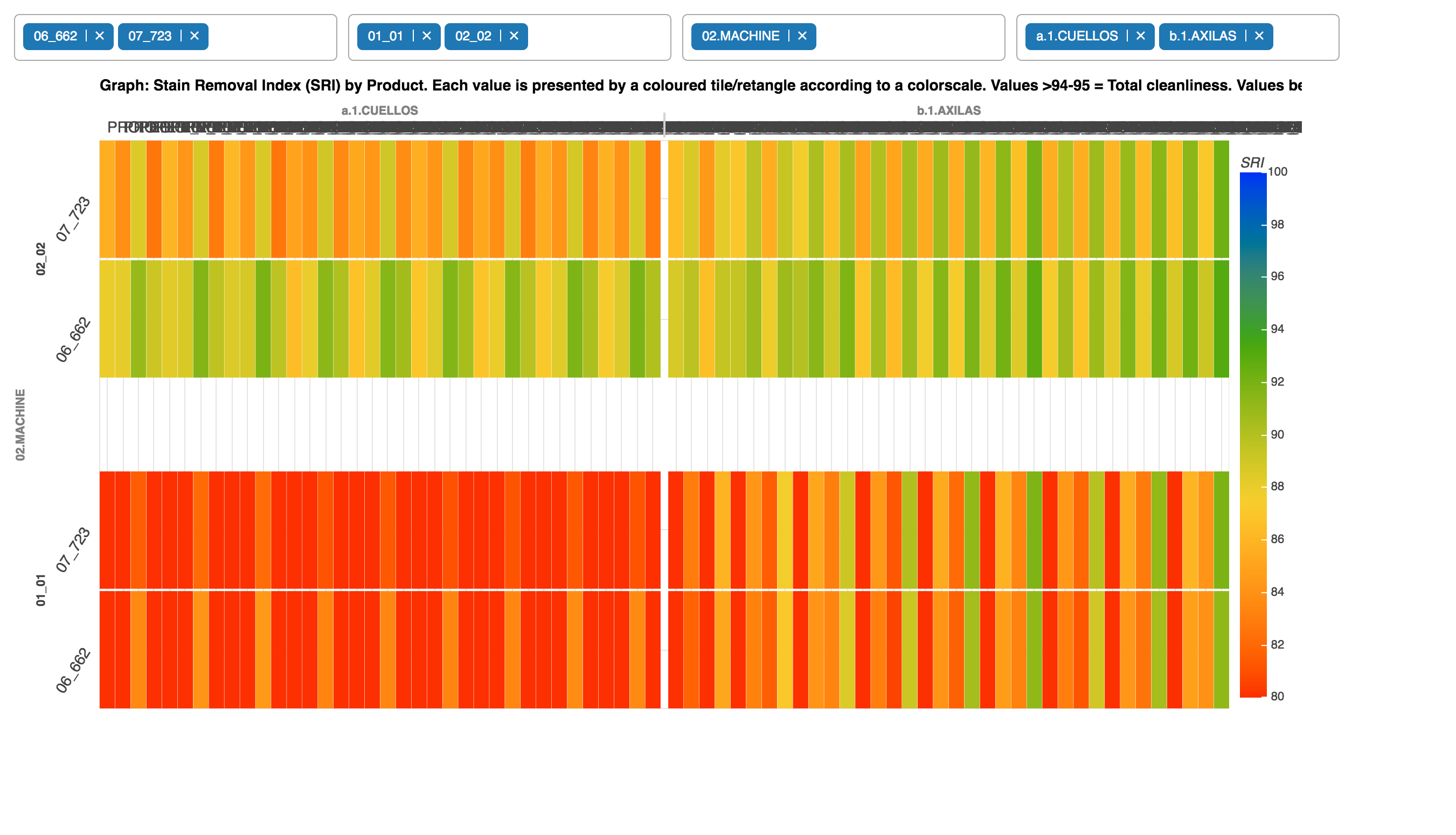
Dear Carolyn. I am working in categorical heatmaps with 2 or 3 categories per axis. All works fine in Bokeh Server, but I decide to build the graphic using CustomJS because unsolved problems during embedding the graph with frameworks. Below is the code that include data so you can reproduce it. Additional comments:
… it is clear that CustomJSFilter and CDSView filter that data since the beginning and data is updated. It means, initial graph depends on the initial values of the widget, which is fine, and data is filtered and changes according to change in multiple selection, which is expected
… the problem is how to synchronize x_range and y_range with data filters, at the beginning and then when multiple selection change.
I am a novice user and expect your kind help.

Rodrigo

import pandas as pd
import numpy as np
import colorcet as cc

from bokeh.plotting import figure, output_notebook, show
from bokeh.layouts import column, layout, row
from bokeh.models import ColumnDataSource, HoverTool, MultiChoice, CustomJSFilter, CDSView, CustomJS, FactorRange, LinearColorMapper, ColorBar, BasicTicker, Title, Div
from bokeh.palettes import Spectral5
from bokeh.palettes import palettes
from bokeh.transform import linear_cmap, factor_cmap, transform

data_array = {‘WASH’: [‘01_01’, ‘01_01’, ‘01_01’, ‘01_01’, ‘01_01’, ‘01_01’, ‘01_01’, ‘01_01’],
‘PROCESS’: [‘02.MACHINE’, ‘02.MACHINE’, ‘02.MACHINE’, ‘02.MACHINE’, ‘02.MACHINE’, ‘02.MACHINE’, ‘02.MACHINE’, ‘02.MACHINE’],
‘PRODUCT’: [‘06_662’, ‘06_662’, ‘06_662’, ‘06_662’, ‘06_662’, ‘06_662’, ‘06_662’, ‘06_662’],
‘MONITOR’: [‘a.1.CUELLOS’, ‘a.1.CUELLOS’, ‘a.1.CUELLOS’, ‘a.1.CUELLOS’, ‘b.1.AXILAS’, ‘b.1.AXILAS’, ‘b.1.AXILAS’, ‘b.1.AXILAS’],
‘DIVERSE_SCENARIOS’: [‘PROPER-FV_2_ILLCFL_30-1.2.SRI_STw’, ‘PROPER-FV_2_ILLCFL_30-2.2.SRI_LIw’,
‘PROPER-FV_2_ILLCFL_30-3.2.SRI_HUw’,
‘PROPER-FV_2_ILLCFL_30-4.2.SRI_CRw’,
‘PROPER-FV_2_ILLCFL_30-1.2.SRI_STw’,
‘PROPER-FV_2_ILLCFL_30-2.2.SRI_LIw’,
‘PROPER-FV_2_ILLCFL_30-3.2.SRI_HUw’,
‘PROPER-FV_2_ILLCFL_30-4.2.SRI_CRw’],
‘SRI’: [78.25, 76.79, 83.55, 76.19, 77.53, 81.73, 79.79, 85.2 ],
‘MON_SCEN’: [(‘a.1.CUELLOS’, ‘PROPER-FV_2_ILLCFL_30-1.2.SRI_STw’),
(‘a.1.CUELLOS’, ‘PROPER-FV_2_ILLCFL_30-2.2.SRI_LIw’),
(‘a.1.CUELLOS’, ‘PROPER-FV_2_ILLCFL_30-3.2.SRI_HUw’),
(‘a.1.CUELLOS’, ‘PROPER-FV_2_ILLCFL_30-4.2.SRI_CRw’),
(‘b.1.AXILAS’, ‘PROPER-FV_2_ILLCFL_30-1.2.SRI_STw’),
(‘b.1.AXILAS’, ‘PROPER-FV_2_ILLCFL_30-2.2.SRI_LIw’),
(‘b.1.AXILAS’, ‘PROPER-FV_2_ILLCFL_30-3.2.SRI_HUw’),
(‘b.1.AXILAS’, ‘PROPER-FV_2_ILLCFL_30-4.2.SRI_CRw’)],
‘PROC_WASH_PROD’: [(‘02.MACHINE’, ‘01_01’, ‘06_662’),
(‘02.MACHINE’, ‘01_01’, ‘06_662’),
(‘02.MACHINE’, ‘01_01’, ‘06_662’)]}

dff_stacked = pd.DataFrame(data=data_array)

source = ColumnDataSource(data=dff_stacked)

########################
########################

START TO GRAPH

l_products = list(dff_stacked.PRODUCT.unique())
l_washes = list(dff_stacked.WASH.unique())
l_processes = list(dff_stacked.PROCESS.unique())
l_monitors = list(dff_stacked.MONITOR.unique())

SET UP WIDGETS AND CALLBACKS

mc_product = MultiChoice(value=list(l_products[:1]), options=l_products, title=“Products / Technologies”, width=570)
mc_wash = MultiChoice(value=list(l_washes[:1]), options=l_washes, title=“Number of washes”)
mc_process = MultiChoice(value=list(l_processes[:1]), options=l_processes, title=“Process / Drying”)
mc_monitor = MultiChoice(value=list(l_monitors[:1]), options=l_monitors, title=“Monitors”, width=1200)

custom_filter = CustomJSFilter(args=dict(moni_choice=mc_monitor), code="""
const indices =
for (var i = 0; i < source.get_length(); i++) {
if (source.data[‘MONITOR’][i] == moni_choice.value
) {
indices.push(true)
} else {
indices.push(false)
}
console.log(source.data[‘MONITOR’][i])
}
console.log(moni_choice.value)
console.log(source.get_length())
console.log(indices)
return indices
“”")

view = CDSView(source=source, filters=[custom_filter])

mc_product.js_on_change(‘value’, CustomJS(args=dict(source=source), code="""
source.change.emit()
“”"))
mc_wash.js_on_change(‘value’, CustomJS(args=dict(source=source), code="""
source.change.emit()
“”"))
mc_process.js_on_change(‘value’, CustomJS(args=dict(source=source), code="""
source.change.emit()
“”"))
mc_monitor.js_on_change(‘value’, CustomJS(args=dict(source=source), code="""
source.change.emit()
“”"))

moni_scen_list = list(np.unique(source.data[‘MON_SCEN’]))
proc_wash_prod_list = list(np.unique(source.data[‘PROC_WASH_PROD’]))

TOOLTIPS = [(‘Scenario’, ‘@DIVERSE_SCENARIOS’), (‘SRI’, ‘@SRI’)]

plot = figure(x_range=FactorRange(*moni_scen_list), y_range=FactorRange(*proc_wash_prod_list), x_axis_location=“above”, toolbar_location=‘below’, tools=“save,hover,pan,wheel_zoom,box_zoom,reset”, tooltips=TOOLTIPS, plot_width=1300, plot_height=550)

mapper = LinearColorMapper(palette=list(reversed(cc.b_rainbow_bgyr_35_85_c72)), low=80, high=100)

plot.rect(x=“MON_SCEN”, y=“PROC_WASH_PROD”, width=1, height=1, source=source, view=view, line_color=None, fill_color=transform(‘SRI’, mapper))

color_bar = ColorBar(color_mapper=mapper, location=(0, 0), ticker=BasicTicker(desired_num_ticks=10), title=‘SRI’)

plot.xaxis.group_label_orientation = ‘horizontal’
plot.xaxis.group_text_font_size = “12px”
plot.xaxis.major_label_text_font_size = “0px”
plot.xaxis.major_label_orientation = 0

plot.yaxis.group_text_font_size = “14px”
plot.yaxis.subgroup_text_font_size = “14px”
plot.yaxis.major_label_text_font_size = “14px”
plot.yaxis.major_label_orientation = “vertical”

plot.x_range.group_padding = 0.5
plot.x_range.factor_padding = 0.02
plot.y_range.group_padding = 0.04
plot.y_range.subgroup_padding = 0.05
plot.y_range.factor_padding = 0.02

plot.add_layout(color_bar, ‘right’)

########################
########################

SET UP FINAL GRAPH

inputs = layout([[mc_product, mc_wash, mc_process],[mc_monitor]])

graph_final = layout(column(inputs, plot))

show(graph_final)

@CONSUMERTEC please edit your post to use the actual code formatting tools, so that the code is intelligible (either with the </> icon on the editing toolbar, or triple backtick ``` fences around the code blocks)