Plot and source data consistency for specialized example with constrained interaction

Hi,

I have an application with two linked plots, one of which supports a point-draw tool to interactively move to a point of interest (similar in behavior to a slider UI in a 1D case, which I’d prefer not to use in my particular end-use scenario).

The second link plot displays data on a constrained curve (or surface) corresponding to that selection.
I apply client-side transforms to enforce the constraints.

The interactions and displays work as expected, but I notice that in general the underlying source data is not guaranteed to be consistent with what is shown on the plot. The mismatch happens when a move or add action puts the point of interest outside of the allowable domain.

Is there a preferred way to achieve the desired consistency for this particular use case?

I am using bokeh 2.0.1 and running as a server. A simple example to illustrate the problem follows, and a screen capture of the simplified illustrative example is attached.

#!/usr/bin/env python3
# -*- coding: utf-8 -*-
"""
"""
import numpy as np

from bokeh.plotting import figure, curdoc
from bokeh.transform import transform

from bokeh.layouts import column

from bokeh.models import LinearInterpolator
from bokeh.models import ColumnDataSource, PointDrawTool


def data_cb(attr, old, new):
    print("X OLD:{:+.3f} NEW:{:+.3f}".format(old['xpt'][0],new['xpt'][0]))


# Constrained point viewer
p0 = figure(x_range=(-1.333,1.333), y_range=(-1.333,1.333), width=500, height=500)
p0.toolbar_location = None

# Linked x- selector figure
p1 = figure(x_range=p0.x_range, y_range=p0.y_range, width=500, height=30, background_fill_color='#000000')

p1.xaxis.major_label_text_color = None
p1.xaxis.major_label_text_font_size = '0pt'

p1.xaxis.ticker.desired_num_ticks = 0
p1.yaxis.ticker.desired_num_ticks = 0

p1.toolbar_location = None


# Quadratic reference curve
xq = np.arange(-1.000,1.001,0.001)
yq = 2.000*(xq ** 2) - 1.000
Sq = ColumnDataSource(data=dict(xq=xq, yq=yq))
p0.line(x='xq', y='yq', source=Sq, line_color='#AAAAAA')

# Point on curve
# Linear interpolators constrain interactive taps to reference curve
li_x = LinearInterpolator(x='xq', y='xq', data=Sq, clip=False)
li_y = LinearInterpolator(x='xq', y='yq', data=Sq, clip=False)

Spt = ColumnDataSource(data=dict(xpt=[xq[500]]))
Spt.on_change('data', data_cb)

r0 = p0.circle(x=transform('xpt', li_x), y=transform('xpt', li_y), source=Spt, size=12, fill_color='#000000', line_color='#000000')
r1 = p1.circle(x=transform('xpt', li_x), y=0.0, source=Spt, size=12, fill_color='#FFFFFF', line_color='#FFFFFF')

_drawtool = PointDrawTool(renderers=[r1], add=True, num_objects=1)

p1.add_tools(_drawtool)
p1.toolbar.active_tap = _drawtool

curdoc().add_root(column(p0,p1))
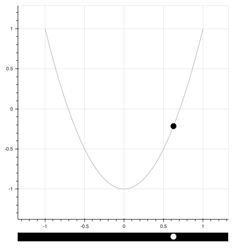
@_jm you are going to have to explain a bit more. I am afraid I don’t understand what inconsistency you are referring to from this description (or from running the code). You say:

I notice that in general the underlying source data is not guaranteed to be consistent with what is shown on the plot.

How exactly is this observed?

Otherwise offhand all I can suggest is that PointDrawTool has no notion of bounds, it will update its CDS with whatever data arises from the interaction. If that’s not what you want, then PointDrawTool is probably not what you want.

Thanks for the quick reply.

In the simplified example, I have an x-axis range (-1.333,1.333). If I use the point-draw tool and click on a point beyond that range, the plots adhere to the constraints I impose to restrict the point to [-1.0,1.0]. I impose these using bokeh’s LinearInterpolator with the clip argument equal False

I observe that the underlying source data is not consistent with the plot via the data_cb callback function, which is registered as an on_change('data', ...) callback for the source.

Here is a representative printout for one such interaction. Note that the new x-value in the source equals a value > 1.000, although the point in the figure is never allowed to go there b/c of the constraints applied.
Basically, the new x-value corresponds to where the mouse was via the completed move or add (drag) action. I guess I’m looking for a way that the transform/clipping of the interpolator can be honored in the source data.

2020-04-09 15:07:56,423 Starting Bokeh server version 2.0.1 (running on Tornado 6.0.4)

2020-04-09 15:07:56,424 User authentication hooks NOT provided (default user enabled)

2020-04-09 15:07:56,426 Bokeh app running at: http://localhost:5006/qex

2020-04-09 15:07:56,426 Starting Bokeh server with process id: 84482

2020-04-09 15:08:01,691 WebSocket connection opened

2020-04-09 15:08:01,692 ServerConnection created

X OLD:-0.500 NEW:+1.201

The following workaround serves the purpose. Basically, a separate source for the two plots is required, and an intermediate callback is used to enforce constraints and restore coupling.

In the end-use application that motivated the topic, the constraints are in lower dimensions (1-D/2-D/3-D) so the overhead of a second data source that honors the constraints is minimal. (The constraint enforcement is important for calculations that operate on the data in a physically achievable domain.)

#!/usr/bin/env python3
# -*- coding: utf-8 -*-
"""
"""
import numpy as np

from bokeh.plotting import figure, curdoc
from bokeh.transform import transform

from bokeh.layouts import column

from bokeh.models import LinearInterpolator
from bokeh.models import ColumnDataSource, PointDrawTool


# Constrained point viewer
p0 = figure(x_range=(-1.333,1.333), y_range=(-1.333,1.333), width=500, height=500)
p0.toolbar_location = None

# Linked x- selector figure
p1 = figure(x_range=p0.x_range, y_range=p0.y_range, width=500, height=30, background_fill_color='#000000')

p1.xaxis.major_label_text_color = None
p1.xaxis.major_label_text_font_size = '0pt'

p1.xaxis.ticker.desired_num_ticks = 0
p1.yaxis.ticker.desired_num_ticks = 0

p1.toolbar_location = None


# Quadratic reference curve
xq = np.arange(-1.000,1.001,0.001)
yq = 2.000*(xq ** 2) - 1.000
Sq = ColumnDataSource(data=dict(xq=xq, yq=yq))
p0.line(x='xq', y='yq', source=Sq, line_color='#AAAAAA')

# Point on curve
# Linear interpolators constrain interactive taps to reference curve
li_x = LinearInterpolator(x='xq', y='xq', data=Sq, clip=False)
li_y = LinearInterpolator(x='xq', y='yq', data=Sq, clip=False)

Spt0 = ColumnDataSource(data=dict(xpt=[xq[500]]))
Spt1 = ColumnDataSource(data=dict(xpt=[xq[500]]))

def lim_cb(attr, old, new):
    print("OP-LIM OLD:{:+.3f} NEW:{:+.3f}".format(old['xpt'][0],new['xpt'][0]))
    op = min(max(new['xpt'][0], -1.0), 1.0)
    data_patch = {}
    data_patch.update(xpt=[(0, op)])
    Spt0.patch(data_patch)

def sel_cb(attr,old, new):
    print("OP-SEL OLD:{:+.3f} NEW:{:+.3f}".format(old['xpt'][0],new['xpt'][0]))
    
Spt0.on_change('data', sel_cb)
Spt1.on_change('data', lim_cb)

r0 = p0.circle(x=transform('xpt', li_x), y=transform('xpt', li_y), source=Spt0, size=12, fill_color='#000000', line_color='#000000')
r1 = p1.circle(x=transform('xpt', li_x), y=0.0, source=Spt1, size=12, fill_color='#FFFFFF', line_color='#FFFFFF')

_drawtool = PointDrawTool(renderers=[r1], add=True, num_objects=1)


p1.add_tools(_drawtool)
p1.toolbar.active_tap = _drawtool

curdoc().add_root(column(p0,p1))
1 Like