Here is a toy example that illustrates the techniques you can use (you will need to adapt them to your specifics)
from bokeh.models import Legend, LegendItem
from bokeh.palettes import Category10_3
from bokeh.plotting import figure, show
from bokeh.sampledata.iris import flowers
from bokeh.transform import factor_cmap, factor_mark
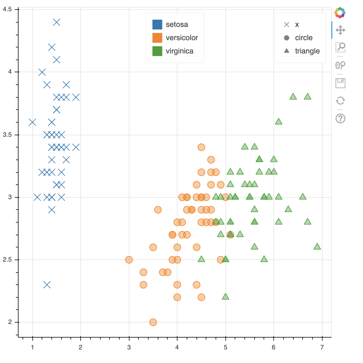
SPECIES = ['setosa', 'versicolor', 'virginica']
MARKERS = ['x', 'circle', 'triangle']
p = figure()
# plot the actual data using factor and color mappers (using the same
# column `species` here but you can use two different columns if you want)
r = p.scatter("petal_length", "sepal_width", source=flowers, fill_alpha=0.4, size=12,
marker=factor_mark('species', MARKERS, SPECIES),
color=factor_cmap('species', Category10_3, SPECIES))
# we are going to add "dummy" renderers for the legends, restrict auto-ranging
# to only the "real" renderer above
p.x_range.renderers = [r]
p.y_range.renderers = [r]
# create an invisible renderer to drive color legend
rc = p.rect(x=0, y=0, height=1, width=1, color=Category10_3)
rc.visible = False
# add a color legend with explicit index, set labels to fit your need
legend = Legend(items=[
LegendItem(label=SPECIES[i], renderers=[rc], index=i) for i, c in enumerate(Category10_3)
], location="top_center")
p.add_layout(legend)
# create an invisible renderer to drive shape legend
rs = p.scatter(x=0, y=0, color="grey", marker=MARKERS)
rs.visible = False
# add a shape legend with explicit index, set labels to fit your needs
legend = Legend(items=[
LegendItem(label=MARKERS[i], renderers=[rs], index=i) for i, s in enumerate(MARKERS)
], location="top_right")
p.add_layout(legend)
show(p)