Square matrix (350x350) + ColorBar

[grzegorz.malinowski]

I’d appreciate any suggestion how to set figure properties to have square matrix (350x350) + ColorBar, that corresponds to the bar chart(350x350).

source = ColumnDataSource(data={'x_axis': X,
                                'y_axis': Y,
                                'data': Z})
p2 = figure(x_range=x_names, y_range=y_names,
            plot_height=350, plot_width=350,
            match_aspect=True)
color_bar = ColorBar(color_mapper=mapper, location=(0, 0))
p2.add_layout(color_bar, 'right')
show(p2)

[Bryan]

@grzegorz.malinowski “corresponds to the bar chart” is very vague and I can think of at least a few different potential interpretations right off the top of my head. You need to be more specific about exactly what it is and what parts you want line up.

[_jm]

@grzegorz.malinowski

Are you saying that you want the topmost figure to be square (350px by 350px) excluding the colorbar sidebar? And additionally you want it to be left and right aligned with the barchart below? If so, do you also want the axes to be aligned, which would imply that the labels of the Y axis would also factor into the solution, I believe.

[grzegorz.malinowski]

Here is the pattern I’d like to achieve. I’d like to control both width and height of both plots. Colorbar is included but not in this 350x350 size. Please take into account that I’d like to have different scales.

[_jm]

@grzegorz.malinowski

You will need to increase the width property of the figure that has the colorbar layout added to it. The colorbar has a settable width (defaults to auto, I believe, but you can prescribe it to something known a priori). The colorbar also has a margin, label_standoff, and the actual label characters that use up space. So, you will need to account for these in the figure width.

If you want to work at a higher level, you can check out Holoviews which plots with bokeh, but lets you set a “square” aspect ratio for the plot. See http://holoviews.org/user_guide/Plotting_with_Bokeh.html

[grzegorz.malinowski]

Ok. Many thanks _jm. I’ll be experimenting with different colorbar parameters then.

BTW

1. Does it mean that aspect_ratio=1 doesn’t work?
2. Does it exist any automatic method to adjust width/height to keep aspect ratio? Even if I could manage to define the correct values it can be easily distorted since the size depends also on axis labeling.

As or me, the best approach would be:
a) define real plot w/h
b) define aspect
c) increase automatically entire plotting area by taking into account all other elements like labels, colorbars, etc.
d) align them based on axis position

[_jm]

@grzegorz.malinowski

I haven’t studied the machinery of the aspect-ratio code, but my interpretation from the documentation is that it is more designed for the use case where a figure is analogous to a single graphical element, e.g. 2-D plot axes only, and doesn’t consider what happens when additional auxiliary objects like color bars or when really verbose labels for major ticks are used.

I personally have encountered scenarios where the problem has required precise aspect ratios to convey certain physical characteristics of the data being presented, and have either resorted to coming up with a scheme to compensate for the real estate lost to that other information or other workarounds (see following basic example to illustrate). The only other option I know of is to look at Holoviews that abstract alot of the low-level controls of Bokeh away from the user but provide controls for such things as square aspect ratios without you having to figure it out as a user.

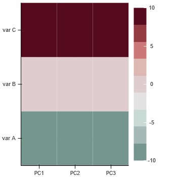
Here’s one option that you might consider. The idea is to create a phantom (hidden) second plot that holds the colorbar so that it doesn’t take up space from the plot area you are actually interested in. It uses the extrema of the data only to minimize the amount of additional data that needs to be plotted while maintaining the colorbar scale of interest. The colorbar is added to the lefthand side of the phantom/hidden plot to make it appear attached to the visible plot.

The most obvious downside of this approach is that it constrains what you can do if you need toolbars. The other issue might be bookkeeping if you are dynamically. and interactively updating the plots.

The main benefit is obviously the avoiding the need for manually adjusting plot width to recover real estate lost to the colorbar.

#!/usr/bin/env python3
# -*- coding: utf-8 -*-
"""
"""
import numpy as np

from bokeh.plotting import figure, show
from bokeh.layouts import row
from bokeh.models import LinearColorMapper, BasicTicker, ColorBar


data = np.random.rand(10,10)

color_mapper = LinearColorMapper(palette="Viridis256", low=0.0, high=1.0)

p = figure(width=350, height=350, x_range=(0.0,1.0), y_range=(0.0,1.0),
           toolbar_location=None)
p.image(image=[data], color_mapper=color_mapper,
        dh=[1.0], dw=[1.0], x=[0], y=[0])


# hidden plot with (min,max) data to support colobar
data_minmax = np.array([[data.min()],[data.max()]])

ph = figure(width=350, height=350, x_range=(0.0,1.0), y_range=(0.0,1.0),
            toolbar_location=None)
imh = ph.image(image=[data_minmax], color_mapper=color_mapper,
               dh=[1.0], dw=[1.0], x=[0], y=[0])

cb = ColorBar(color_mapper=color_mapper, ticker= BasicTicker(),
               location=(0,0))
ph.add_layout(cb, 'left')

# Hide
ph.xaxis.visible = False
ph.xgrid.visible = False

ph.yaxis.visible = False
ph.ygrid.visible = False

ph.outline_line_color = None

imh.visible = False

show(row([p,ph]))

[grzegorz.malinowski]

Thank you _jm. I really appreciate your help. Holoview looks promising and seems is the solution (for matrix like this - correlation - hover tool is rather necessary). Eh, another library to be familiar with.

[Bryan]

Another suggestion: if your primary concern is that inner frame widths matching up, rather than both inner frames matching exactly, then you could put the color bar on the top or the bottom, and give both plots the same min_border_left and min_border_right values that are large enough to accommodate whatever the larger axis is.

[grzegorz.malinowski]

To and for developers.

Is anyone able to produce sth like this? Would solve many problems with aspect_ratio.

How can I set the aspect ratio in matplotlib?

/section Original Answer:/

[grzegorz.malinowski]

I’m not 100% sure but seems that the below is Bokeh solution
frame_height=
frame_width=
match_aspect=