Bokeh Developers,
I could not find a simple streaming sine wave example that did not rely on database, threading, or Javascript.
So, here is a complete, stand-alone time series plotting example for live streaming data.
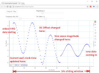
This example generates a sine wave and displays it using a first-in-first-out (FIFO) buffer that makes the sine wave appears to slide, or move along the time axis. New data enters on the right and the oldest data exits on the left.
It has buttons and sliders for user input, a pause button, and also uses Bokeh’s inspection tools with the reset button.
It has a live updating annotation in the plot window showing elapsed time from the browser session and iteration index.
This is similar to surface3d example with periodic updates suitable for bringing in live streaming data.
This is a self-contained function for use in Bokeh 0.12.6 and probably more recent.
Run with:
bokeh serve --show streamingSine.py
This is a sample screenshot:
Here’s the code:
from bokeh.layouts import column, widgetbox, layout
from bokeh.models import Button, Label, HoverTool
from bokeh.models.widgets import Slider
from bokeh.palettes import RdYlBu3
from bokeh.plotting import figure, curdoc
from bokeh.driving import count
from collections import deque
import numpy as np
import time
initialize an empty double-ended queue to grow x and y arrays as new data comes in
new_data_x = deque()
new_data_y = deque()
------------------------------------------------------------------------------------------
user-defined parameters
T_update = 100 # (ms) browser update rate specified in add_periodic_callback()
timeWindow = 14 # (s) time window to display
nMax = timeWindow/(T_update/1000) # number of datapoints at specified sample rate to achieve time window in seconds
#nMax=10
i = 0
t0=time.time() # (s) initialize t0 with seconds since the epoch, 01 Jan 1970 (a giant number, like 1500157344.7670777)
------------------------------------------------------------------------------------------
BEGIN: update_window()
update_window(y,u,N) creates a FIFO window of the most recent data, moving in time as updates occur
streamingSine.py (6.17 KB)
···
this function accepts a deque list, y, and additional scalar data point u,
and appends u to deque list y until length reaches N.
When y is length N, drop the oldest in y and add u.
uses native python double ended queue’s (deque’s) to avoid creation of new
numpy arrays or shifting the entire python list each iteration
def update_window(y,u,N):
if len(y)<N:

    y.append(u) # append to the right side of the deque list (this is the newest, or entering data)

else:

    y.append(u) # append 1 number to the right side (this is the newest, or entering data)

    y.popleft() # remove 1 number from the left side (this is the oldest, or exiting data)


return y
END: update_window()
------------------------------------------------------------------------------------------
create a plot and style its properties
plot = figure( # x_range=(-10, 10), y_range=(-10, 10),
       tools="pan,xpan,ypan,hover,crosshair,box_zoom,reset,save",

       x_axis_label='my X-axis', y_axis_label='my Y-axis', plot_height=500, plot_width=900)
plot.border_fill_color = ‘white’
plot.background_fill_color = ‘white’
plot.outline_line_color = ‘LightBlue’
plot.grid.grid_line_color = ‘LightBlue’
add a text renderer to our plot
http://bokeh.pydata.org/en/latest/docs/reference/models/annotations.html
label = Label(x=50, y=50, text=" i={0:d}, t={1:0.2f}(s)".format(0,0),
          text_font_size='11pt', border_line_color='black', background_fill_color='white',

          x_units='screen', y_units='screen',#level='glyph', render_mode='css',

          background_fill_alpha=0.8, text_color='blue') # text_color='#eeeeee'
plot.add_layout(label)
make some sliders to vary sine wave magnitude, frequency, and vertical offset
sliderMag = Slider(start=0, end=10, value=5, step=2, title=“Magnitude”)
sliderFreq = Slider(start=0.1, end=0.5, value=0.2, step=0.1, title=“Frequency (Hz)”)
sliderOffset = Slider(start=-5, end=+5, value=0, step=1, title=“DC Offset”)
add a circle renderer with a size, color, and alpha: http://bokeh.pydata.org/en/latest/docs/reference/plotting.html
series = plot.circle(x=, y=, size=4, color=‘blue’, fill_alpha=0.2)
ds = series.data_source
------------------------------------------------------------------------------------------
callback for da Start/Stop button, add_periodic_callback() is what makes this loop
def callback_button():
global t0

if button.label == 'Press to: > Play':

    button.label = 'Press to: = Pause'

    curdoc().add_periodic_callback(callback_update_data, T_update) # <-- this controls update frequency

    #t0=time.time() # (s) reset base time, t0, each time button is pressed

else:

    button.label = 'Press to: > Play'

    curdoc().remove_periodic_callback(callback_update_data)
------------------------------------------------------------------------------------------
------------------------------------------------------------------------------------------
@count()
create a callback that will add a number from a networked data source (this example creates y=Asin(omegat) )
def callback_update_data(t):
global i,t0,new_data_x,new_data_y


i = i + 1

t = time.time()-t0 # (s) system time, real wall-clock time in seconds since the epoch, minus t0 is elapsed time in seconds


# create a new dictionary each loop iteration

new_data = dict()


#y = update_window(y,u,N) # grow a deque to size N then update as a FIFO buffer for a sliding window with newest data

new_data_x = update_window(new_data_x,t,nMax) # append the 't' to new_data_x deque


# create a y value as a function of time - this could easily come from a udp packet sent from the data source

A      = sliderMag.value    # sine wave magnitude

freq   = sliderFreq.value   # sine wave frequency

offset = sliderOffset.value # sine wave vertical offset

y = [A*np.sin(2*np.pi*freq*t) + offset][0] # y=A*sin(omega*t)+offset, omega=2*pi*freq, omega in rad/s, freq in Hz


new_data_y = update_window(new_data_y,y,nMax) # append this loop's y value to new_data_y deque


new_data['x'] = list(new_data_x) # convert double-ended queue into a list, stored as a new dict() entry

new_data['y'] = list(new_data_y)

ds.data = new_data # BEST PRACTICE --- update .data in one step with a new dict


# dynamically update label text

label.text = " i={0:10d}, t={1:10.3f}(s)".format(i,time.time()-t0)
------------------------------------------------------------------------------------------
add a button widget and configure with the call back
button = Button(label=‘Press to: > Play’, width=100)
button.on_click(callback_button)
put the button and plot in a layout and add to the document
layout = layout([
[widgetbox(button),widgetbox(sliderMag)],

[widgetbox(sliderFreq),widgetbox(sliderOffset)],

[plot],
], sizing_mode=‘fixed’) # “fixed”, “stretch_both”, “scale_width”, “scale_height”, “scale_both”
curdoc().add_root(layout)
curdoc().title = “streamingSine example”
``
